Continuing on with the Kylerec posts… (see the first one here as well as notes to follow along with here).
This post is a synthesis of the following talks:
- Day 1 Talk 2 – François-Simon Fauteux-Chapleau’s talk on Weinstein handles and contact surgery
- Day 1 Talk 3 – Orsola Capovilla-Searle’s talk on Kirby calculus for Stein manifolds
- Day 1 Talk 4 – Alvin Jin’s talk on Lefschetz fibrations and open books
- Day 2 Talk 1 – Bahar Acu’s talk on mapping class factorizations and Lefschetz fibration fillings
- Day 3 Talk 2 – Sarah McConnell’s talk on applications of Wendl’s theorem to fillings
- Day 5 Talk 1 – Ziva Myer’s talk on flexible and loose Legendrians
Weinstein surgery theory
I assume the reader is familiar with smooth surgery theory. Recall the following definition.
Definition: A Weinstein cobordism consists of a quadruple  , where
 is a compact symplectic manifold with boundary
 is a Liouville vector field for , meaning
  , which is also transverse to the boundary
 is a Morse function
- is gradient-like for
 , meaning there is some constant
  with
with  with respect to a given Riemannian metric.
In this case, the boundary decomposes as  , where points out of
  and into
  . Note that the 1-form
  satisfies
  , and is sometimes called the Liouville 1-form, since it encodes the same data as . Also note that a Weinstein cobordism with
  is what we called a Weinstein filling.
The gradient-like condition is meant to give some directionality (since  ) and ensure that the critical points of are non-degenerate. One typically doesn’t think of the precise choice of pair
  as very important, but rather the data up to some notion of homotopy. For example, one can always perturb the Morse function so that each of and is a regular -level set, regardless of the number of components, and so we might as well assume this from the start. The equivalence hinted at here is called Weinstein homotopy, by which we perturb the pair , possibly through birth-death type singularities.
Lemma: The descending manifolds in a Weinstein cobordism, i.e. the set of points which flow along to a given critical point in infinite time, are isotropic submanifolds.
Proof: Standard Morse theory implies these submanifolds are smooth. Let  be the flow along at time
  , and suppose we choose some
  where
where  is some descending manifold for a given critical point
  . Suppose
  is a vector in the tangent space. Then since
  , we have that

As  , the right hand side goes to zero since
  for all
  in a curve
  along with tangent vector
  at
at  . Hence,
  , from which it follows that
  . Hence,
  , and so also
  .
.
Corollary: All critical points in a Weinstein cobordism  are of index at most
  . Smoothly, any such manifold can be built up by surgery starting from a neighborhood of
  and attaching handles of index at most .
One would like to be a bit more precise about how the surgery interacts with the symplectic geometry. As a first step, along a regular level set  , the symplectic condition on
  implies that
  is a contact form. The proof of the lemma above further implies that
  gives an isotropic submanifold of
  with respect to .
So we can think, at least smoothly, that our Weinstein cobordism is built up, starting from , by attaching handles with isotropic cores and attaching spheres along isotropics in level sets of (which are contact submanifolds). But there’s a little more that we know about neighborhoods of isotropics. In a symplectic manifold, the neighborhood of an isotropic  is completely determined up to symplectomorphism by its symplectic normal bundle,
  , as a symplectic vector bundle (with symplectic structure induced by on the fibers). A similar statement holds for isotropic submanifolds in contact manifolds, but now with their neighborhoods determined up to contactomorphism by the conformal symplectic normal bundle
  , where
  is a contact form so that
  is symplectic on
  . Furthermore, if we fix , then the symplectic vector bundle structure determined by on the nose determines the neighborhood up to exact contactomorphism. Patching these two things together, one finds:
Theorem [Weinstein, before the term “Weinstein handle” was coined]: Weinstein handle attachment is completely specified (up to Weinstein homotopy) by matching the symplectic framing data determined by  along the isotropic attaching spheres.
One therefore thinks of as being built up from by contact surgery along isotropic submanifolds with given framing information compatible with the underlying symplectic topology.
Consider a Weinstein cobordism of dimension  . Then the handles of index
  are called subcritical handles, whereas the handles of index
  are called critical handles. When , the aformenetioned symplectic normal bundles are trivial automatically, and so one specifies critical handle attachment simply by drawing a Legendrian sphere on .
Recall that the proof of the h-cobordism theorem requires some ability to cancel (and create) pairs of handles with index differing by 1 whose ascending and descending manifolds intersect in a 1-dimensional manifold, to move around attaching spheres, and to move critical values around. The last of these we can always do, so we can attach the handles in order of their index. It turns out that when  , we can recreate all parts of the proof of the h-cobordism theorem for subcritical Weinstein cobordisms. In some sense, subcritical Weinstein domains have no symplectic geometry in them – they are encoded by algebro-topological information, and so this gives some flexibility phenomena.
It turns out that some critical handles behave the same way. The key obstruction to the aforementioned flexibility is that sometimes the data of an attaching Legendrian does not boil down to purely toplogical information. However, Emmy Murphy defined a class of Legendrians, called loose Legendrians, for which there is such a so-called h-principle. The Weinstein h-cobordism theorem works for Weinstein cobordisms which can be built (up to Weinstein homotopy) out of subcritical and loose critical handle attachments. We call such Weinstein cobordisms flexible.
We often care about the case when  . In this case, it is pretty easy to describe a connected Weinstein domain (or its contact boundary). One can first order the handles by index, and then cancel 0-handles with 1-handles until we are in the situation where there is precisely one 0-handle and possibly many 1- and 2-handles. The boundary of the 0-handle is just a standard contact
  , and 1-handle attachment is trivially described by picking pairs of points in (the bundle data boils down to showing
  ). So it suffices to draw Legendrians on with
  pairs of points identified, which is just
  . Any Legendrian
  has a canonical framing of its normal bundle given by the twisting of the Reeb chord around the Legendrian. Eliashberg showed that adding a left twist to this framing gives the smooth framing which determines the corresponding smooth surgery data.
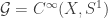
Gompf showed that in this case , one can draw standard Kirby calculus type surgery diagrams. We think of all of these 1-handle attachments and Legendrians as missing a point in , so that we can draw our diagrams in  . The front projection is the projection to the coordinates
  , so that
  is determined by
  . It might not be obvious how to draw a smooth knot in this projection since the curve can’t have infinite slope, but we are allowed semi-cubical cusps, corresponding to
  . Note that transverse crossings are also allowed, since the -coordinates are distinct. One usually draws the front projection of a Legendrian without showing which strand lies over the other, but we include this extra information in the next figure, where we imagine the -axis as pointing into the page.

A Legendrian trefoil knot
Gompf’s standard form for these Legendrians looks like the following, where the pairs of balls in each row corresponds to where the 1-handles are attached, and the Legendrian strands simply go through the handles as though they were wormholes.
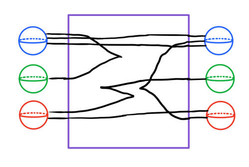
An example of a Gompf surgery diagram. There are three 1-handles (in blue, red, and green) and two 2-handles with attaching spheres given by the Legendrian tangle above. All of the information can be made to live inside of the purple rectangle (i.e. without going horizontally or vertically outside of where the 1-handles are attached).
Weinstein fillings, Lefschetz fibrations, and open book decompositions
Definition: A Lefschetz fibration is a smooth map  with finitely many critical points with distinct critical values such that locally around the critical points,
  looks like a complex Morse function (i.e.
  in local coordinates). When
  has boundary, we assume the critical values of are all in the interior of .
We shall typically be concerned with the case where  (although see this post by Laura Starkston which slightly generalizes some of what is discussed here).

A schematic for a Lefschetz fibration over the disk
In the case where , we see that the boundary decomposes as  , where the superscripts are meant to indicate vertical and horizontal. That is,
  , while
  . If we write
  for a regular fiber of , then
  . Meanwhile, we see that
  is just a fibration over
  with fiber , and hence can be described by some monodromy map
  fixing the boundary, so that
 ![\partial^v W = F \times [0,1]/{\sim}](https://s0.wp.com/latex.php?latex=%5Cpartial%5Ev+W+%3D+F+%5Ctimes+%5B0%2C1%5D%2F%7B%5Csim%7D&bg=ffffff&fg=333333&s=0&c=20201002) where
where 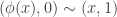 (the mapping torus of ).
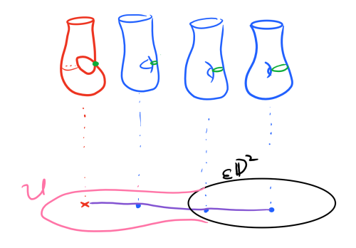
The structure on the boundary, in which we have a fibration over with fiber glued together with  in the natural way, is called an open book decomposition. It is given completely by the pair
  . We think of each fiber over as a page, and the subset
  as the binding, analogous to what one would get if one took their favorite book and matched the covers so that the pages radiate outwards. So Lefschetz fibrations yield open books on the boundary. To be a little more precise, one should extend each page so that the boundary of each page is actually the binding.

Some pages near the binding of an open book. I guess the name “Rolodex” wasn’t as catchy as “open book.” (Image from Wikipedia)
Now suppose  is a regular value (which can always be arranged up to small perturbation of ). Then
 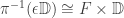 . One can ask what happens when we extend to
  , where
  and there is exactly one critical value on
  .
.
Since we have a nice fibration away from critical points, we see that paths in  yield monodromy maps (up to isotopy preserving boundary) on the fibers. We can choose a connection on the fibration if we wish to make this a map on fibers, not just a map up to isotopy. If we take a path from 0 to which intersects
  once and otherwise avoids critical values then for whatever connection we chose, we can see what points flow to the critical point over . Over each regular fiber, this is just a circle, and the union of all of them together with the critical point yields a disk. The path is called a vanishing path, and each circle on the regular fiber is called a vanishing cycle (one really should think of it as a homology cycle, but for concreteness, one can think of it as a curve). The disk consisting of the union of vanishing cycles above a path is called a thimble.
The green circles in the regular fibers above the purple vanishing path are the vanishing cycles. Their union is the thimble.
It is then not hard to see that is obtained from  by 2-handle attachment, where the attaching curve is just the vanishing cycle above
  and the core of the handle is the thimble. Furthermore, one can check by a local computation that the monodromy map in a loop around is just given by a Dehn twist (positive or negative, depending on orientations) around the vanishing cycle. Hence, one can write out the open book determined by the Lefschetz fibration explicitly – it is just the product of the Dehn twists on the vanishing cycles, performed in an order determined by a sequence of vanishing paths.
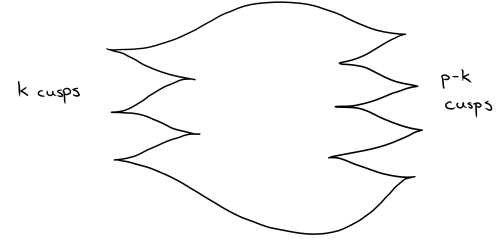
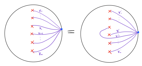
Notice that for a given regular value on  , one can choose a different basis of vanishing paths, and this yields a possibly different factorization for the monodromy. Such changing of the basis is generated by so-called Hurwitz moves, as drawn below.
Hence, understanding Lefschetz fibrations over the disk essentially corresponds to understanding factorizations of mapping class group elements into Dehn twists.
Now, this whole story can be repeated in the symplectic context, as follows.
Definition: A symplectic Lefschetz fibration is a Lefschetz fibration with a symplectic manifold such that each fiber is symplectic submanifold away from the critical points, while at the critical points the coordinates in which locally looks like a complex Morse function can be taken to be holomorphic for some compatible almost complex structure  .
.
In this case, one can take the connection to be the symplectic connection given the symplectic orthogonal complement to the vertical directions. In this way, the thimbles produced will actually be Lagrangian disks, which suggests one can think of these as the descending disks for a Weinstein domain filling the boundary. In addition, the monodromy maps are now compositions of positive Dehn twists only, since the symplectic condition gives the proper orientations. In other words, our Lefschetz fibration is itself positive. If the vanishing cycles of a Lefschetz fibration are homologically nontrivial, we shall call it allowable.
With a little more work, we can obtain the following theorem of Loi and Piergallini (although an alternative proof by Akbulut and Özbağci is more in line with the exposition presented here):
Theorem: Any positive allowable Lefschetz fibration (PALF) yields a Weinstein domain, and any Weinstein domain comes from a PALF in this way.
Furthermore, one obtains a little bit more compatibility at the boundary.
Definition: An open book decomposition on a manifold  is said to support a cooriented contact structure if there is some contact form for such that the binding is a contact submanifold, is a symplectic form on the pages, and the boundary orientation of the page (with respect to ) matches the orientation of the binding with respect to .
One checks that the open book on the boundary of a PALF does indeed support the contact structure determined by being the boundary of a Weinstein domain.
Our surgery theory for these Lefschetz fibration builds the fiber up by subcritical surgery, and the 2-handle attachments correspond to the critical points of the fibration. One can always produce, for any Weinstein manifold, a cancelling pair consisting of a 1-handle and a 2-handle. The way that this affects the open book is by positive stabilization, meaning that one adds a 1-handle to the page, but kills it by adding an extra Dehn twist to the monodromy through a circle which passes through the handle.
The following theorem implies that all 3-dimensional contact geometry can actually be encoded (somewhat non-trivially) in the study of open books up to positive stabilization, and hence the study of Weinstein fillings reduces to studying positive factorizations of given elements of the mapping class group of a surface with boundary (up to this not-so-easy-to-work-with notion of positive stabilization).
Theorem [Giroux correspondence]: There is a one-to-one correspondence between contact structures on a closed 3-manifold up to isotopy with open books up to positive stabilization.
Applications to Weinstein fillings
To summarize the previous section, an explicit surgery decomposition of a Weinstein filling yields a PALF which in turn gives an open book structure supporting the contact boundary of the Weinstein filling with monodromy factored into positive Dehn twists. Conversely, given a supporting open book for a contact structure with monodromy factored into positive Dehn twists, one obtains a Weinstein filling.
One common question we ask is whether a single contact manifold has multiple Weinstein fillings. From the above construction, one possible way to attack this problem is to look for distinct positive factorizations of a given element in a mapping class group.
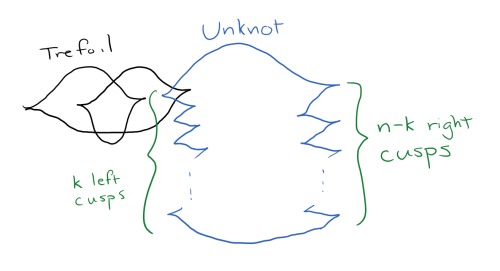
Theorem [Auroux]: There is an element in the mapping class group of the surface  (of genus 1 and with one boundary component) with two distinct factorizations into positive Dehn twists such that the Weinstein fillings are distinguished by their first homology.
Remark: In this setting, the first homology is just given by  where is the span of the vanishing cycles. The only real trick of Auroux is therefore to find a good candidate for the above theorem to hold, and just compute.
Generalizing a bit more:
Theorem [Baykur – Van Horn-Morris]: There exists an element in the mapping class group of  (of genus 1 with three boundary components) which admits infinitely many positive factorizations such that the corresponding Weinstein fillings are all distinguished from each other by their first homology.
Finally, as one last application, I want to consider a result of Plamenvskaya and Van Horn-Morris, but I need to define the contact structures in question to begin. Honda’s classification of tight contact structures on the lens spaces  can be formulated in Gompf’s surgery diagrams by the following diagrams, coming from a single 2-handle attachment to standard . We denote the corresponding contact structures by
  .
.
The surgery diagram for the contact structure  .
.
Of these, the universal covers of  and
and  are also tight, where as the others’ universal covers are overtwisted. We say
  are virtually overtwisted.
Theorem [PV]: Each virtually overtwisted  has a unique Weinstein filling (up to symplectic deformation) and a unique minimal weak filling.
Proof sketch: Let us first discuss the Weinstein part. There are a few nontrivial theorems which go into this, which we won’t discuss, but essentially we have the following sequence of results. The open book given by the surgery diagrams above induce open books with genus 0 pages. When we discussed Wendl’s theorem in part 2 of the J-holomorphic curve posts, one thing we mentioned was that one can apply his techniques when there is a planar open book (meaning pages have genus 0). He proves that if a contact manifold has a given supporting planar open book, then every Weinstein filling is diffeomorphic to one compatible with that specified planar open book. Hence, it suffices to study Lefschetz fibrations compatible with the one just described, which in turn becomes studying factorizations of an element in the mapping class group of  , the disk with holes. A nontrivial result of Margalit and McCammond gives that every such presentation must be in a certain form, from which one can use smooth Kirby calculus to conclude that the surgery diagram must come from
  -surgery on some knot. Finally, an appeal to work of Kronheimer, Mrowka, Ozsváth, and Szabó using Seiberg-Witten Floer homology (also called monopole Floer homology) yields that this knot must have been an unknot, and since the framing is , this determines the canonical framing of the knot, which in turn implies we could only have had one of our original surgery diagrams.
Finally, to obtain the weak part, one can use work of Ohta and Ono to boost a weak filling up to a strong filling, from which Wendl’s theorem implies that any minimal weak filling is symplectic deformation equivalent to a Weinstein filling.


(meaning
where
is the Hodge star with respect to
)
-structure


![c_1(X,\omega)[\omega] < 0](https://s0.wp.com/latex.php?latex=c_1%28X%2C%5Comega%29%5B%5Comega%5D+%3C+0&bg=ffffff&fg=333333&s=0&c=20201002)


![c_1(X) \cdot [\omega] = 0](https://s0.wp.com/latex.php?latex=c_1%28X%29+%5Ccdot+%5B%5Comega%5D+%3D+0&bg=ffffff&fg=333333&s=0&c=20201002)


 th and
  st critical points. Note that the corresponding vanishing cycles for the critical point corresponding to
  and
and  are actually different, but the overall monodromy on the open book at the boundary is the same.
 . The idea was that if we had a filling
  , then the presence of an overtwisted disk locally gave a Bishop family of holomorphic disks as part of a 1-dimensional moduli space, but the compactified moduli space was seen to have only one boundary point. This was because continuing the family away from the center of the overtwisted disk could not lead to a possible boundary point – in our version, such a point would require a bubble, but we considered exact fillings.
 is the symplectic manifold
  , where
  -coordinate. This symplectic manifold does not depend upon the choice of
  , then
  where
where  sending
  .
. -bundle over
  . Fixing a local section
  for the fiber such that the symplectic form is just
  . We simply take the component where
  and
and 
 is a compatible almost complex structure for
 on which there is nontrivial behavior, where
  remains fixed but
  . In the limit, as these two intervals get farther apart, we break into two holomorphic curves in the symplectization. This forms what is sometimes called a holomorphic building. In general, there may be multiple levels in the limit, as in the figure below.
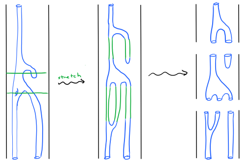
![((-\epsilon,0] \times M, d(e^t\alpha))](https://s0.wp.com/latex.php?latex=%28%28-%5Cepsilon%2C0%5D+%5Ctimes+M%2C+d%28e%5Et%5Calpha%29%29&bg=ffffff&fg=333333&s=0&c=20201002) where
where  , to form a completed symplectic manifold
  . I can choose some compatible almost complex structure
  . In this case, one can study J-holomorphic curves, and we have a similar Gromov compactness statement. In this case, our curves can either bubble, or form holomorphic buildings where the lowest level is just
  and whose higher levels are all
  .
. ).
). of the moduli space containing a special leaf in the symplectization end. This component is 2-dimensional, and hence is precisely given by the foliating leaves around it (recall
  , where the fibers are symplectic (since they are J-holomorphic and
  ) and generically smooth except with finitely many nodal singular fibers, forming what is called a symplectic Lefschetz fibration.
 ? The answer is yes in the case when
  (with contact structure induced by the restriction of the Liouville form on
  to the unit cotangent bundle). In this case, any strong filling, not just the standard one, would have
 ![\overline{\mathcal{M}_0} = [0,1] \times S^1](https://s0.wp.com/latex.php?latex=%5Coverline%7B%5Cmathcal%7BM%7D_0%7D+%3D+%5B0%2C1%5D+%5Ctimes+S%5E1&bg=ffffff&fg=333333&s=0&c=20201002) , and so any strong filling of
, and so any strong filling of ![[0,1] \times S^1](https://s0.wp.com/latex.php?latex=%5B0%2C1%5D+%5Ctimes+S%5E1&bg=ffffff&fg=333333&s=0&c=20201002) . Wendl then beefs this up to prove, for example, that every minimal strong filling of
. Wendl then beefs this up to prove, for example, that every minimal strong filling of  .
. satisfying some conditions. If there is some other leaf
  which is not diffeomorphic to
 ![([0,1] \times T^2, \cos(2\pi t)d\theta_1 + \sin(2\pi t)d\theta_2)](https://s0.wp.com/latex.php?latex=%28%5B0%2C1%5D+%5Ctimes+T%5E2%2C+%5Ccos%282%5Cpi+t%29d%5Ctheta_1+%2B+%5Csin%282%5Cpi+t%29d%5Ctheta_2%29&bg=ffffff&fg=333333&s=0&c=20201002) , obstructs fillability, originally
, obstructs fillability, originally  have a surgery theory consisting of handles of index at most
  . The main theorem states that the existence of just one subcritical Weinstein filling places restrictions on the topology of any strong symplectically aspherical filling
  .
. admitting a subcritical Stein filling with the homotopy type of a CW complex of dimension
  , then any strong symplectically aspherical filling
  for
for  via the isomorphism induced by inclusion
 otherwise
 , then all strong aspherical fillings of
  , McDuff’s theorem from last time about fillings of lens spaces implies that there is a unique minimal filling up to diffeomorphism. By positivity of intersection, symplectically aspherical fillings are minimal, which implies the above result. But also, since
  a Liouville manifold of finite type (meaning it is modelled after a positive symplectization outside of some compact region). Let
  be the corresponding Liouville vector field (satisfying
  ). The
  in
in  such that:
 where
where  is the standard radial Liouville vector field on
 is modelled after the positive symplectization of
 replaced with
  ).
). is
is  -spliffable, and using smooth topology.
 of a closed manifold
  admits no subcritical Weinstein fillings.
 surjects onto
  with
with  . This is a contradiction.
 so that it is convex (which we can do by the spliffability condition). The interior component determine by the splitting through
  such that the interior embeds diffeomorphically onto
  . This embedding then gives us a smooth manifold
  which looks like
  but with the interior component replaced by
  .
.
 , where
  is admissible (as discussed in the previous section) for
  such that
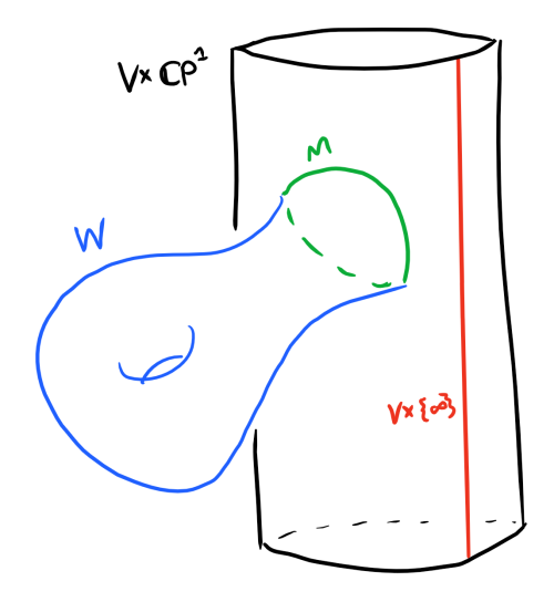
 ![[u] = [\{v\} \times \mathbb{C}P^1]](https://s0.wp.com/latex.php?latex=%5Bu%5D+%3D+%5B%5C%7Bv%5C%7D+%5Ctimes+%5Cmathbb%7BC%7DP%5E1%5D&bg=ffffff&fg=333333&s=0&c=20201002) (for some
(for some  ,
,  , and
, and  , for some choice of
  distinct and not
  .
. .
. . First of all,
  . This map is actually proper and degree 1, which follows from the maximum principles just described, plus a little boost from positivity of intersection which implies that there is no need to worry about stable maps in the compactification of
  .
.

 which is right inverse to
  on the level of homology).
 . Given an almost complex manifold, a J-holomorphic curve is a map
  such that
  is a Riemann surface and
  . In the case where
  is a complex manifold, we see this is precisely what it means to be holomorphic.
 . By this, we mean that the (0,2)-tensor
  is a Riemannian metric. We say
  for each nonzero vector
  factors as
  such that the first map is a branched cover of Riemann surfaces. J-holomorphic curves which are not multiply covered are called simple, and it turns out that simple curves are characterized by being somewhere injective, meaning there is some
  for which
  and
and  . Even better, somewhere injective means that
  is almost everywhere injective.
 the moduli space of all simple
 ![u_*[\Sigma]](https://s0.wp.com/latex.php?latex=u_%2A%5B%5CSigma%5D&bg=ffffff&fg=333333&s=0&c=20201002) of the map
of the map  to some
  . The main question is:
 actually a smooth manifold?
 , where
  .
. where
where  is a biholomorphism. A more careful author would probably distinguish between the map
  by reparametrization to obtain moduli spaces of curves. Usually, these are the main objects of interest.
 has an energy
  attached to it (when
  given by
  . We see that away from
  , this is just converging to the curve
  . But near
  , if we reparametrize the domain by
  , we see this converges to the sphere
  .
. given by
  , in which a new bubble forms at
 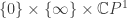 in addition to the one discussed above. More generally, a sequence of curves can limit to a curve with trees of bubbles sticking out.
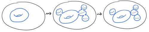
 (modulo reparametrization of domain) can be compactified by adding in stable curves of total energy bounded by
  in the homology class
 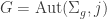 is the group of biholomorphisms of
  . Then the group
  acts on
  by
by 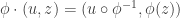 . Notice then that the evaluation map
  only depends on the orbit, and hence descends to a map
  . Proving enough properties of such an evaluation map sometimes allows us to compare the smooth topology of
  is a simple J-holomorphic curve representing the class
  with geometric self-intersection number
  , then
 .
. , such that the so-called characteristic foliation
  on
on  , which is actually a singular foliation, looks like the following image, with one singular point in the center and a closed leaf as boundary.
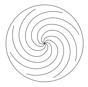
 . We study the space of certain J-holomorphic disks with boundary on the overtwisted disk. The key is that a neighborhood of the overtwisted disk
  actually has a canonical neighborhood in
  , with its standard contact structure given by the complex tangencies, i.e.
 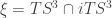 , with
  . Then consider the disk given by
  . The characteristic foliation on this disk looks like the characteristic foliation near the center of the overtwisted disk, so a neighborhood of this disk in
  yields a model for a neighborhood of the center of the overtwisted disk. We may assume the almost complex structure in this neighborhood is just given by the standard one,
 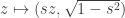 for
for  a real constant near 0. That these are all of the somewhere injective disks is a relatively easy exercise in analysis. Namely, suppose we had such a disk of the form
  . Then since boundary points are mapped to the overtwisted disk,
  . But each component of
  is harmonic, hence satisfies a maximum principle. Therefore,
  . But by holomorphicity,
  is real, so we can draw this situation in
  by forgetting the imaginary part of
 . This is by a maximum principle which comes from analytic convexity properties of a filled contact manifold.
 . But one checks that the relation
  implies that for a
  , we have
  . This vanishes by Stokes’ Theorem since
  is exact, and so
  such that
  is a smooth closed symplectic 4-manifold and
  . We call a rational curve
  with respect to the intersection product on
  (with respect to its orientation coming from
  contains no exceptional curves. The main theorem is as follows:
 , then
  , in which case
  is an integer. Let us first define this contact structure. Recall that the standard contact structure on
  where the action of
  given by
  preserves the contact structure, so that it descends.
 , these fillings are unique up to diffeomorphism, and further up to symplectomorphism upon fixing the cohomology class
 ![[\omega]](https://s0.wp.com/latex.php?latex=%5B%5Comega%5D&bg=ffffff&fg=333333&s=0&c=20201002) . The space
. The space  has two nondiffeomorphic minimal fillings.
 over
over  for any such given
 ![[C]](https://s0.wp.com/latex.php?latex=%5BC%5D&bg=ffffff&fg=333333&s=0&c=20201002) can be represented by a
can be represented by a  , where:
![A_i := [S_i]](https://s0.wp.com/latex.php?latex=A_i+%3A%3D+%5BS_i%5D&bg=ffffff&fg=333333&s=0&c=20201002) is
is  must actually be a legitimate curve of one component)
 are distinct and embedded curves of self-intersection -1, 0, or 1, with at least one index for which
  .
. and
and  , then it had already been shown that this implies that
  . This bleeds into…
 consisting of simple holomorphic spheres representing the class
 ![A = [S]](https://s0.wp.com/latex.php?latex=A+%3D+%5BS%5D&bg=ffffff&fg=333333&s=0&c=20201002) . This comes with an evaluation map of the form
. This comes with an evaluation map of the form
 and we have positivity of intersection. Therefore, this map has degree 1, and so any pair of distinct points on
  is a simple homology class in
  , and suppose
  with symplectic fibers and such that
  of rational embedded
  , and where
 ![d = \dim V + 2c_1(TV) \cdot [C] - 4](https://s0.wp.com/latex.php?latex=d+%3D+%5Cdim+V+%2B+2c_1%28TV%29+%5Ccdot+%5BC%5D+-+4&bg=ffffff&fg=333333&s=0&c=20201002) ,
, fixing the marked point. Applying adjunction for the curve represented by
 ![[C] \cdot [C] = 0](https://s0.wp.com/latex.php?latex=%5BC%5D+%5Ccdot+%5BC%5D+%3D+0&bg=ffffff&fg=333333&s=0&c=20201002) , yields
, yields  . We also have an evaluation map
 where the fibers are precisely the curves in our moduli space. Since the fibers are holomorphic, they are symplectic by the taming condition.
 has a structure group which can be reduced to
  , but the complex bordism group is well known to satisfy
  . As a consequence, every contact manifold is smoothly fillable. We must therefore consider fillability questions which extend beyond the realm of complex bordism in order to discover interesting phenomena.
 such that
  . There is a generalization in higher dimensions due to
  is
is  is strongly fillable if there is a weak filling
  such that one can find a Liouville vector field
  gives a (properly cooriented) contact form for
  where
where  .
. on
on  and
and  fits into an exact triangle with Morse homology, and so one can understand the topology of a filling from its symplectic homology. One might be interested, for example, in studying fillings with
  , in which case the homology of the filling is completely determined by