Monthly Archives: July 2017

by ksackel | July 10, 2017 · 11:09 pm

Kylerec – Seiberg-Witten and Fillings

The first post on Kylerec is here, so if you haven’t been keeping up with these posts, you might want to start there. This is also the last post on the Kylerec 2017 workshop, which has been fun and rewarding to write about (with some much appreciated help from Agustín Moreno)!

If you’re following along with the lecture notes from Kylerec, then this post corresponds to Day 4 (Talks 11-14), consisting of the following four talks:

My talk following sections 2-3 of Hutchings and Taubes Introduction to the Seiberg-Witten equations.
Jie Min’s talk, on section 4 of those notes (the symplectic manifold case), but also continuing on to Morgan and Szabó’s paper which can be used to classify homotopy K3 surfaces
Tom Gannon’s talk on fillings of unit contangent bundles, following Li-Mak-Yasui and Sivek–Van Horn-Morris
Dani Álvarez-Gavela’s talk on how Lisca and Matić distinguish contact structures using Seiberg-Witten theory

A pre-introduction to Seiberg-Witten theory

The Seiberg-Witten equations have been discussed in this blog by Laura Starkston in a sequence of four posts. For more information, details, and clarification, the interested reader should go there, or to the notes of Hutchings and Taubes mentioned in the introduction to this post. I call this a pre-introduction because the details will be rather sketchy. I will not even write the Seiberg-Witten equations down. The reader interested in skipping to fillings may wish to jump ahead to the two-sentence summary at the end of this section.

I should mention that the Seiberg-Witten equations arise naturally in physics, although I’ve not yet personally taken the time to understand Witten’s motivation for first writing down these equations, which he called the monopole equations. If you are interested in that sort of thing, maybe check out this MathOverflow post.

Consider a closed oriented smooth 4-manifold $X$ , together with the following data:

a Riemannian metric $g$
a self-dual 2-form $\mu$ (meaning $*\mu = \mu$ where $*$ is the Hodge star with respect to $g$ )
a $\textbf{spin}^c$ -structure $\mathfrak{s} \in \mathcal{S}_X$

You might be asking – what’s a $\text{spin}^c$ -structure? Recall that for $n \geq 3$ , one has $\pi_1(\text{SO}(n)) = \mathbb{Z}/2\mathbb{Z}$ , so one can form the connected double cover $\text{Spin}(n)$ . Then one defines the Lie group

$\text{Spin}^c(n) = (\text{Spin}(n) \times U(1))/ \pm 1.$

This comes with a map to $\text{SO}(n)$ with fiber $U(1)$ . The metric $g$ yields a principal $\text{SO}(n)$ -bundle called the frame bundle, which topologically doesn’t depend on the metric, and a $\text{spin}^c$ -structure is just a principal $\text{Spin}^c(n)$ -bundle such that quotienting by the $U(1)$ -action (sitting inside the $\text{Spin}^c(n)$ -action) recovers the frame bundle.

For $X^4$ oriented, which is the case of interest to us, the space of $\text{spin}^c$ -structures, $\mathcal{S}_X$ , is an affine space modelled on $H^2(X;\mathbb{Z})$ (this is not obvious). Also in the 4-dimensional case, representation theory of the Lie group $\text{Spin}^c(4)$ yields two complex 2-dimensional spinor bundles $S_{\pm}$ and a complex line bundle $L = \det S_{\pm}$ . The Seiberg-Witten equations are then equations on pairs $(A,\psi)$ consisting of a $U(1)$ -connection on $L$ and a positive spinor (a section of $S_+$ ). We write this simply as

$\mathcal{F}_{g,\mu,\mathfrak{s}}(A,\psi) = 0$ .

Let $\mathfrak{m}_{g,\mu,\mathfrak{s}}$ be the solutions to this eqution. There is an action of the gauge group $\mathcal{G} = C^{\infty}(X,S^1)$ (given by $h \cdot (A,\psi) = (A-2h^{-1}dh,h\psi)$ ). This action is free except for reducible solutions where $\psi = 0$ , in which case the stabilizer is $S^1$ . The quotient yields the moduli space (where we suppress $g,\mu,\mathfrak{s}$ from the notation):

$\mathcal{M} = \mathfrak{m}/\mathcal{G}$

Theorem (key, nontrivial): The space $\mathcal{M}$ is always compact.

Let $b_2^+$ be the rank of the positive-definite part of $H^2(X;\mathbb{R})$ with respect to the intersection product. We will assume $b_2^+ > 1$ . This implies that generically paths of choices $(g,\mu)$ for a fixed $\mathfrak{s}$ will avoid reducible solutions, yielding the following.

Theorem (standard Fredholm theory): Consider $X$ with $b_2^+ > 1$ and some fixed $\mathfrak{s}$ . Then generically (with respect to $(g,\mu)$ ),

$\mathcal{M}$ is a smooth finite-dimensional manifold of dimension given by topological data (only depending on $X$ and $\mathfrak{s}$ )
$\mathcal{M}$ can be given an orientation with some auxiliary topological choice (not depending on $\mathfrak{s}$ )
$\mathcal{M}$ is a cobordism invariant

Definition: For $b_2^+ > 1$ , and for $\mathfrak{s}$ with $\dim \mathcal{M} = 0$ , we define the Seiberg-Witten invariant $\text{SW}_X(\mathfrak{s}) = \#\mathcal{M} \in \mathbb{Z}$ , where we count $\mathcal{M}$ with signs according to the auxiliary topological choice.

One can also define the Seiberg-Witten invariant when the dimension is positive, but there is the simple type conjecture that in such cases, this invariant is zero. In the case of symplectic manifolds, which is the case we care about, this is known to be true (by Taubes). By construction, the Seiberg-Witten invariants are diffeomorphism invariants (once we have fixed our auxiliary data for determining an orientation of $\mathcal{M}$ ).

We are interested in the case of symplectic manifolds. In this case, there is a canonical choice for the data which orients the moduli spaces of solutions to the Seiberg-Witten equations. There is a natural morphism $\mathcal{S}_X \rightarrow H^2(M;\mathbb{Z})$ given by the $c_1(L)$ where $L$ is the line bundle mentioned before. (This is not an isomorphism if $H^2(X;\mathbb{Z})$ has 2-torsion.)

Definition: A class $c \in H^2(M;\mathbb{Z})$ is basic if there is a $\text{spin}^c$ -structure $\mathfrak{s}$ with $c_1(L_{\mathfrak{s}}) = c$ such that $\text{SW}_{X}(\mathfrak{s}) \neq 0$ .

We finish by stating the following facts without proof (although we did discuss the proofs at Kylerec).

Theorem [Taubes]: For a symplectic manifold, $\pm c_1(X,\omega)$ are basic classes (with Seiberg-Witten invariants $\pm 1$ ).

Theorem [Corollary of the same Taubes paper]: When $(X,\omega)$ is minimal, Kähler, and of general type (the last condition meaning $c_1(X,\omega)[\omega] < 0$ and $c_1^2(X,\omega) > 0$ ), then $\pm c_1(X,\omega)$ are the only basic classes.

Theorem [Corollary of Morgan-Szabó]: If $(X^4,\omega)$ has $c_1(X,\omega) = 0$ , $b_1 = 0$ , and $b_2^+ > 1$ , then it is a rational homology K3 surface.

SUMMARY OF THIS SECTION: The Seiberg-Witten invariants form a diffeomorphism invariant, hence so do basic cohomology classes. This fact, plus the previous three theorems, are all we need.

Filling unit cotangent bundles

Unit cotangent bundles, which we shall notate as $S^*M$ , have canonical Weinstein fillings given by the unit disk cotangent bundles. It is a natural question to ask if this natural filling is in fact the only one up to some notion of equivalence. We shall restrict ourselves in this discussion to when the base space is a closed orientable surface $\Sigma_g$ of genus $g$ . We mostly focus on the $g \geq 2$ case, but we quickly review the case of $g = 0,1$ .

Let us begin with $g=0$ . In the first post on J-holomorphic curves, when discussing McDuff’s classification result, I mentioned that $L(2,1) = S^*S^2$ has a unique minimal strong filling up to diffeomorphism. Further, Hind proved that Stein fillings are unique up to Stein homotopy.

For $g=1$ , in the second post on J-holomorphic curves, when discussing Wendl’s J-holomorphic foliations, I mentioned that every minimal strong filling of $S^*T^2$ to the standard one. In fact, he proves further that every minimal strong filling is symplectically deformation equivalent, which is a little stronger. Also, Stipsicz proved that all Stein fillings are homeomorphic (to $D^*T^2 = D^2 \times T^2$ ).

To summarize roughly (though we know a little more), for $g=0,1$ , exact fillings (which are automatically minimal) are unique up to symplectic deformation equivalence.

So now we move on to $g \geq 2$ . We focus on exact fillings because strong fillings (even minimal ones) are too weak to get a handle on. One can build strong fillings with arbitrarily large positive second Betti number $b_2^+$ . This involves cutting out a cap (with concave boundary) from one particular strong filling (McDuff) and gluing in other caps with higher $b_2^+$ (Etnyre and Honda).

The idea, in this paper of Li, Mak, and Yasui, is similar to the idea we encountered in McDuff’s approach to the $g=0$ (and more generally $L(p,1)$ ) case – attach a cap, and then use classification results to figure out what you had in the first place. The following definition is the correct version of cap that we need.

Definition: A Calabi-Yau cap for a contact 3-manifold $(M,\xi)$ is a strong cap (like a filling, but with a concave end instead) $(P,\omega)$ with $c_1(P,\omega)$ torsion.

Theorem 1 [LMY]: If a Calabi-Yau cap exists for $(M,\xi)$ , then the set of triples of Betti numbers $(b_1(X), b_2(X), b_3(X))$ is finite as $X$ ranges over all exact fillings.

Remark: This theorem is not true if instead we let $X$ range over all strong fillings. This was noted above when we remarked that $b_2^+$ could be arbitrarily large for a strong filling.

Theorem 2 [LMY]: In the case of the unit cotangent bundle, then for any exact filling $(X,\omega)$ , its homology $H^*(X;\mathbb{R})$ and intersection form $H^2(X;\mathbb{R}) \otimes H^2(X, \partial X;\mathbb{R}) \rightarrow \mathbb{R}$ are the same as that of the standard filling.

Sketch Proof of Theorem 1: Some messing around with Chern classes tells us that if we have an exact filling $(X,\omega_X)$ and a Calabi-Yau cap $(P,\omega_P)$ for $(M,\xi)$ , then the glued manifold $(Z,\omega)$ satisfies $c_1(X) \cdot [\omega] = 0$ . Then one can plug this into classification theorems by an invariant called the symplectic Kodaira dimension $\kappa^s(Z,\omega)$ . In the case when $X$ is minimal with $c_1(X) \cdot [\omega] = 0$ , we must have $\kappa^s = 0$ . In this case, when $b_1 = 0$ , then the Morgan-Szabó result mentioned in the Seiberg-Witten section implies that we have a rational K3 surface, hence we know its Betti numbers. Tian-Jun Li extended this result to a classification for $\kappa^s = 0$ and $Z$ minimal but with arbitrary $b_1$ . Otherwise, if $X$ is not minimal, it must have $\kappa^s = - \infty$ , and one needs to be a little more careful, working with a symplectic surface in $P$ to which an adjunction inequality ends up bounded the Betti numbers.

Sketch Proof of Theorem 2: The key lemma is to construct a symplectic K3 surface $(X,\omega)$ with $g$ non-intersecting Lagrangian tori in the same homology class which all intersect a Lagrangian sphere transversely in one point. Then we can perform Lagrangian surgery to give an embedded Lagrangian genus $g$ surface $L$ . Then $X \setminus \text{Op}(L)$ is a Calabi-Yau cap for $S^*\Sigma_g$ . Playing around with intersection forms, we see that attaching this cap must yield a rational K3 surface (one can rule out all other possibilities given by the classification theorems mentioned in the proof of Theorem 1), from which playing around more with exact sequences of homology and intersection forms gives the result.

Remark: The classification-type results with respect to symplectic Kodaira dimension are the only place in this section where Seiberg-Witten equations enter the picture, and are really the meat of the argument, in some sense. The rest just comes from exact sequences and understanding intersection forms, which is comparatively simple, staying far away from gauge theory.

The main theorem of Sivek and Van Horn-Morris is the following:

Theorem [SV]: Weinstein fillings of $S^*\Sigma_g$ are unique up to s-cobordism rel boundary.

If you’re worried about the word “s-cobordism,” just think of this as a beefed up version of homotopy equivalence that comes relatively easily in this case once we prove the homotopy type of the filling is unique (is a $K(\pi_1(\Sigma_g),1)$ ). There are some beautiful group-theoretic arguments which go into this argument, but we have essentially already seen how the Seiberg-Witten invariants come into play, so I won’t include a sketch of the proof.

Finally, I mention a little bit of history with regards to these two papers, because I was confused looking at the most recent versions as I was writing this, not for lack of improper attributions, just by my own confusions about reading them concurrently. The theorems stated are quite similar, as are aspects of the proofs, despite them being stumbled upon independently. To clarify, Theorem 2 of LMY did not exist in version 1 of their paper. About a year later, within a month of each other, SV posted their paper and LMY posted version 2 of their paper. Independently, SV had proved some subset of Theorem 2 (with some small fudge factor in $H_1$ and the intersection form) while LMY had proved the full version. SV’s result was good enough for them to prove the s-cobordism statement, and as far as I can tell, version 2 of SV is just version 1 but where they mention that they have learned that LMY proved the strong version of Theorem 2.

Homotopic tight contact structures which are different

The main theorem, due to Lisca and Matić, is the following:

Theorem [LM]: For any $n \geq 0$ , there exists a rational homology 3-sphere with at least $n$ distinct contact structures up to contactomorphism which are homotopic as plane fields.

In this short section, we simply sketch the proof.

Sketch of proof: One must begin by simply writing the Gompf surgery diagrams (described in the post on Weinstein fillings) for the contact structures in question. One has that a rational homology sphere can be obtained by 0-surgery on a trefoil and $-n$ -surgery on an unknot which links with the trefoil once, and so suggests the following surgery diagrams so that the canonical framing on the Legendrians drawn below gives exactly what we want.

LM_Surgery

We denote these contact structures by $\xi_n^k$ for $1 \leq k \leq n-1$ . We will show that for a fixed $n$ , all of these are homotopic but not contactomorphic. One computes via results of Eliashberg that for the corresponding Weinstein fillings $W_n^k$ (which are diffeomorphic) that $c_1(W_n^k) = (2k-n)\text{PD}(T)$ , where $T$ is the class in $H_2(W_n^k)$ given by the handle coming from the trefoil in the surgery. We shall call the smooth underlying manifold $N_n$ .

The homotopic part is rather simple. By classical results (clutching functions, and computing Pontrjagin classes to plug into the Hirzebruch signature theorem) following an argument attributed to Gompf, one can show that the homotopic result can be reduced to proving that $c_1(W_n^k)^2 = c_1(W_n^{k'})^2$ , which is itself clear since $\text{PD}(T)^2 = 0$ .

As for the contactomorphism part, one embeds $W_n^k$ into a minimal compact Kähler surface $S$ of general type and $b_2^+ > 0$ . This is a nontrivial statement, but is nonetheless true. In fact, because $W_n^k$ and $W_n^{k'}$ have isomorphic collars, one can attach the same cap to produce Kähler surfaces $S_n^k$ and $S_n^{k'}$ . One can extend the identity on these caps to an orientation preserving diffeomorphism $\phi \colon S_n^k \cong S_n^{k'}$ acting by $\pm 1$ on $H^2(N_n) \subset H^2(S_n)$ (by work of Gompf). But also, since we have a minimal compact Kähler manifold, by the theorem mentioned in the first section as a corollary of Taubes’ work, one has that $\{\pm c_1(S_n^k)\}$ is a diffeomorphism invariant, and so we see that $c_1(S_n^k) = \pm \phi^*c_1(S_n^{k'})$ . So these must restrict to the same thing on $H_2(N_n)$ , where we showed $c_1(S_n^k)|_{H_2(N_n)} = (2k-n) \text{PD}(T)$ . Hence, $2k-n = \pm (2k'-n)$ , so either $k = k'$ or $k = n-k'$ . Thus, increasing $n$ , we can find arbitrarily many homotopic but non-contactomorphic contact structures.

Kylerec – Day 5

SH & SH^+ [Momchil Konstantinov’s talk]

Let us begin with a rather informal and sketchy overview of the basics behind symplectic homology (this is by no means the most general version, and we refer the reader to the vast and growing literature, of which we give some references below).

Consider $(V,\lambda)$ a Liouville domain with contact boundary $(M=\partial V, \alpha= \lambda\vert _{\partial V})$ and its completion $(\widehat{V},\widehat{\lambda})$ , obtained from $(V,\lambda)$ by attaching cylindrical ends. Given a nondegenerate Hamiltonian $H:S^1\times \widehat{V}\rightarrow \mathbb{R}$ , we have an associated action functional 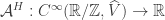$\mathcal{A}^H: C^\infty(\mathbb{R}/\mathbb{Z}, \widehat{V})\rightarrow \mathbb{R}$ , defined by

$\mathcal{A}^H(x)=\int_{S^1}x^*\widehat{\lambda}-\int_{S^1}H_t(x(t))dt$

Its differential is given by $d_x\mathcal{A}^H(\xi)=\int_{S^1}d\lambda(\xi(t),\dot{x}(t)-X_{H_t}(x(t)))dt$ , and it follows that its critical points correspond to closed Hamiltonian orbits. Given a $d\lambda$ -compatible almost complex structure $J$ which is cylindrical on the ends, this induces a metric on the loop space, for which the gradient of $\mathcal{A}^H$ can be written as 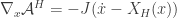$\nabla_x\mathcal{A}^H=-J(\dot{x}-X_H(x))$ , so that the gradient flow equation becomes the Floer equation. We define the symplectic homology chain complex (with mod 2 coefficients) as

$CF_*(H)=\bigoplus_{x \in \mbox{crit}(\mathcal{A}^H)}\mathbb{Z}_2.x$

By simplicity, assume that $x \in \mbox{crit}(\mathcal{A}^H)$ is contractible (so that we don’t have to worry about homology classes and whatnot), and also assume that $c_1(V)=0$ (this condition can be relaxed to $c_1\vert_{\pi_2(V)}=0$ , and is needed for the grading). Then we can define the Conley-Zehnder index of $x$ by choosing spanning disks for $x$ and trivializing $TV$ along this disk, and we choose the grading 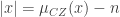$|x|=\mu_{CZ}(x)-n$ , which is independent on the trivialization by the assumption on $c_1(V)$ . The differential is now $d_H: CF_k(H)\rightarrow CF_{k-1}(H)$ , given by

$d_H(x)=\sum_{\substack{y\in \mbox{crit}(\mathcal{A}_H)\\|y|=|x|-1}}\#_{\mathbb{Z}_2}\mathcal{M}(y,x)y$

where $\mathcal{M}(y,x)$ is the moduli space of Floer trajectories joining $x$ to $y$ divided by the natural $\mathbb{R}$ -translation action. This moduli space is a zero dimensional manifold when $|y|=|x|-1$ (for generic $J$ ). Recall that Gromov compactness requires uniform $C^0$ -bounds (which in our situation are not for free, since $\widehat{V}$ is non-compact) and uniform energy bounds (which we have for $u \in \mathcal{M}(y,x)$ , since $E(u)=\mathcal{A}^H(x)-\mathcal{A}^H(y)$ ).

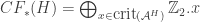
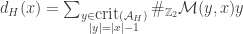
Def. The spectrum of $(M,\alpha)$ is

$spec(M,\alpha)=\{ T \in \mathbb{R}: \mbox{ there exists a }\alpha-\mbox{Reeb orbit of period }T\}$

Def. The space of admissible Hamiltonians $Ad(V,\lambda)$ is the set of Hamiltonians $H: S^1 \times \widehat{V}\rightarrow \mathbb{R}$ satisfying

$H_t(r,y)=Ae^r+B$ on $r>R>>0$ , for some $R$ , where $A>0, A \notin spec(M,\alpha)$ .

Denote by $h(s)=As+B$ , so that $H_t(r,y)=h(e^r)$ on the ends.

If one chooses an admissible $H$ and a $J$ which is cylindrical on the ends, one gets $C^0$ -bounds, as follows from the maximun principle: indeed, consider $\Omega \subseteq \mathbb{R}\times S^1$ an open subset, and $u: \Omega \rightarrow \widehat{V}$ a holomorphic map, which has a portion lying on the cylindrical ends. This portion can be parametrized by $u(s,t)=(a(s,t),v(s,t))\in \mathbb{R} \times M$ , and a computation gives

$\Delta a + \partial_s(h^\prime(e^a))=\Delta a + h^{\prime\prime}(e^a)e^a\partial_sa=||\partial_s v ||^2\geq 0$

The maximum principle then implies that a sequence of Floer cylinders with fixed asymptotics cannot escape to infinity, since we would get a maximum of $a$ , which implies $\Delta a\geq 0$ , and this cannot happen if one assumes that the maximum is non-degenerate (a clever trick then gets rid of this assumption). So we get the $C^0$ -bounds, which leads to compactness by Gromov, which implies $d_H$ well-defined and $d_H^2=0$ (as follows by studying the boundary of 1-dimensional moduli spaces of Floer trajectories). From this, one gets the Floer homology group

$HF_k(H):=H_k(CF_*(H),d_H)$

The first thing one asks is: is it independent of $H$ ? And the answer is…well… nope. BUT…

Consider two different 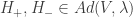$H_+, H_- \in Ad(V,\lambda)$ , and choose a smooth path of Hamiltonians $H^s:\widehat{V}\rightarrow \mathbb{R}$ for $s \in \mathbb{R}$ , such that $H^s=H_-$ for $s<<0$ , $H^s=H_+$ , for $s>>0$ , and $H^s(r,y)=h_s(e^r)=A_se^r+B_s$ for $A_s,B_s \in \mathbb{R}$ , on the cylindrical ends. This gives the parametrized Floer equation $\partial_su + J(\partial_tu - X_{H^s}(u))=0$ and a corresponding moduli space $\mathcal{M}_{\{H^s\}}(x_-,x_+)$ joining the orbits $x_-$ and $x_+$ , which is zero dimensional when $|x_-|=|x_+|$ (now we don’t have a translation action). This ideally would allow us to define a map

$\Phi: CF_*(H_+)\rightarrow CF_*(H_-)$

given by

$\Phi(x_+)=\sum_{\substack{x_- \in \mbox{crit}(\mathcal{A}_H)\\ |x_-|=|x_+|}} \#_{\mathbb{Z}_2} \mathcal{M}_{\{H_s\}}(x_-,x_+)x_-$

satisfying $d_{H_-}\circ \Phi = \Phi \circ d_{H_+}$ , as follows by studying how trajectories in 1-dimensional moduli spaces can break. But this, again, requires Gromov compactness. A similar computation gives

$\Delta a + \partial_s(h_s^\prime (e^a))=\Delta a + h_s^{\prime\prime}(e^a)e^a\partial_sa + (\partial_s h_s^\prime)(e^a)=||\partial_s v||^2$

So, to have $\Delta a + h_s^{\prime\prime}(e^a)e^a\partial_sa\geq 0$ it suffices with

$\partial_sh_s^\prime=\partial_s A_s<0$

In other words, the slope of $H_-$ is necessarily steeper than that of $H_+$ . This means that we only get compactness in “one direction”, and we do not get a homotopically inverse map.

If we define a partial order $\prec$ on $Ad(V,\lambda)$ by $H_1\prec H_2$ if $H_1<H_2$ outside of a compact set, the previous discussion gives us a map $HF_*(H_1)\rightarrow HF_*(H_2)$ . Moreover, we get commutative diagrams for any $H_1 \prec H_2 \prec H_3$ , giving a direct system, so that we may define the symplectic homology of $(V,\lambda)$ as

$SH_k(V,\lambda)=\varinjlim_{H \in Ad(V,\lambda)} HF_k(H)$

Observe that, as with any direct limit, one can compute it by taking cofinal sequences. Now we identify the generators of this homology. Let us recall the following fact from Floer theory:

Fact. If $H$ is sufficiently $C^2$ -small then all the 1-periodic orbits of $X_H$ are critical points of $H$ , and every Floer trajectory between them is a Morse flow-line.

This means that if $H$ is sufficiently $C^2$ -small and positive on $V$ , then the generators on this region of $SH_k$ will correspond to critical points (graded by $|x|=\mu_{CZ}(x)-n=n-ind_x(H)-n=-ind_x(H)$ ), and observe that $\mathcal{A}^H(x)=-H(x)<0$ . On the cylindrical ends, we have $X_H=h^\prime(e^r)e^{-r} R_\alpha$ , where $R_\alpha$ is the Reeb vector field of $\alpha$ on $r=0$ , so that closed Hamiltonian orbits lie in the contact slices $\{r=r_0\}$ and are reparametrizations of closed Reeb orbits of period $T:=h^\prime(e^{r_0})$ , and these have action

$\mathcal{A}^H(x)=T-h(e^{r_0})>0$

Since we assume that the slope of $H$ does not lie in the spectrum, there are no closed orbits for $r>R>>0$ , and between $0$ and $R$ we see potential closed Hamiltonian orbits of bounded action. Since the differential decreases action, we have a subcomplex $CF_*^{-}(H)$ of $CF_*(H)$ generated by orbits of negative action (critical points), and an exact sequence of chain complexes

$0\rightarrow CF_*^{-}(H)\rightarrow CF_*(H)\rightarrow CF_*^+(H)\rightarrow 0$

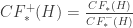where $CF_*^+(H)=\frac{CF_*(H)}{CF_*^{-}(H)}$ . If we define

$SH_*^+(H)=\varinjlim_{H \in Ad(V,\lambda)}H_*(CF_*^+(H),d_H)$

and we take direct limit in the resulting long exact sequence (which preserves exactness), we get an induced exact triangle

diagram

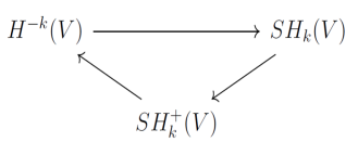
Here we have used the Floer theory fact, and the maximum principle, to say that $CF_*^-(H)$ computes $H^{-k}(V)$ for every $H$ ( $C^2$ -small on $V$ ). Observe that we get cohomology of $V$ rather than homology, since we get a minus in the grading ( $-ind_x(H)$ goes to $-ind_x(H)-1=-(ind_x(H)+1)$ under the differential). Yes, it’s confusing.

We can now state a few theorems.

Thm. [Bourgeois-Oancea] If all Reeb orbits of $(M,\alpha)$ satisfy

$\mu_{CZ}(x)+n-3>0$

that is, if $(M,\alpha)$ is dynamically convex, and $V,W$ are two Liouville fillings of $M$ with $c_1(V)=c_1(W)=0$ , then $SH_*^+(V)\simeq SH_*^+(W)$ .

In other words, $SH_*^+$ is an invariant of $M$ , rather than the fillings (with $c_1=0$ ). The idea is to show that no critical points can be connected to a non-constant orbit by a Floer trajectory, and that no cylinder connecting two of the latter ventures into the filling $V$ (there is a stretching the neck argument here).

Thm. [ML Yau] If $(M,\xi)$ is subcritically Stein fillable (for a filling with $c_1=0$ ), then $M$ admits a dynamically convex contact form.

Thm. [Cieliebak] If $V$ is subcritically Stein (with $c_1=0$ ), then it has vanishing symplectic homology.

Cieliebak proves that $V$ is isomorphic to a split Stein manifold $W \times \mathbb{C}$ , for $W$ Stein, and using a version of the Künneth formula for $SH_*$ , the result follows from the fact that $SH_*(\mathbb{C})=0$ , which one can compute by hand.

Cor. If $V,W$ are subcritical Stein fillings of $(M,\xi)$ with $c_1(V)=c_1(W)=0$ , then $H^*(V)\simeq H^*(W)$ .

This follows from the exact triangle, and all theorems stated above, since $H^{-*}(V)\simeq SH^+_*(V)$ for a subcritical Stein manifold with $c_1(V)=0$ .

References

A few references on symplectic homology (by all means very much non-exhaustive):

A begginer’s overview: https://www.mathematik.hu-berlin.de/~wendl/pub/SH.pdf

A nice survey: https://arxiv.org/abs/math/0403377

A Morse-Bott version (relevant for Cédric’s talk below): https://arxiv.org/abs/0704.1039

A related theory (Rabinowitz Floer homology): https://arxiv.org/abs/0903.0768

Contact manifolds with flexible fillings [Scott Zhang’s talk]

The main reference for this post is this paper: https://arxiv.org/pdf/1610.04837.pdf.

Let us recall the following result, which appeared in Momchil’s talk:

Thm. [M.L Yau] If $W_1, W_2$ are two subcritical fillings of a contact manifold $(M^{2n-1},\xi)$ , (with $c_1(W_1)=c_1(W_2)=0$ ) then $H^*(W_1)\simeq H^*(W_2)$ .

The goal for this talk was to discuss the following generalization to the $\emph{flexible}$ case:

Thm 1. [O. Lazarev] If $W_1,W_2$ are two flexible fillings of $(M,\xi)$ , then $H^*(W_1)\simeq H^*(W_2)$ .

Remark: The same conclusion is true if we consider fillings with vanishing symplectic homology.

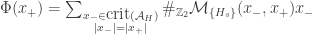
The idea is to replace the dynamical convexity condition in Bourgeois-Oancea’s result by an asymptotic version. In the following, given $\alpha_1,\alpha_2$ contact forms for the same contact structure, we will denote $\alpha_1\geq \alpha_2$ if $\alpha_1=f \alpha_2$ for some smooth function $f\geq 1$ , and by $\mathcal{P}^{<D}(M,\alpha)$ the set of $\alpha$ -Reeb orbits $\gamma$ with action $\int_\gamma \alpha <D$ . The degree of a Reeb orbit $\gamma$ is $|\gamma|=\mu_{CZ}(\gamma)+n-3$ .

Def. $(M^{2n-1},\xi)$ is asymptotically dynamically convex (ADC) if there exists a sequence of contact forms $\alpha_1\geq \alpha_2\geq \dots$ for $\xi$ and a sequence $0<D_1<D_2<\dots$ with $\lim_{i}D_i=\infty$ such that every element in $\mathcal{P}^{<D_i}(M,\alpha_i)$ has positive degree.

We have the following:

Thm 2. [O. Lazarev] If $(M,\xi)$ is ADC, then $SH^+$ is independent of the Stein filling with $c_1=0$ .

Recall that flexible Weinstein manifolds have vanishing symplectic homology. This follows by the Bourgeois-Ekholm=Eliashberg surgery formula (https://arxiv.org/pdf/0911.0026.pdf), but there are alternative arguments not using the SFT machinery, based on an h-principle for exact codimension zero embeddings, and the Künneth formula for symplectic homology, which even works for twisted coefficients (see e.g. Murphy-Siegel https://arxiv.org/abs/1510.01867). From the exact triangle for $SH_+$ , we know that $SH_*^+(W)\simeq H^{-*}(W)$ for flexible $W$ , so to get thm. 1 it suffices to show that flexible fillings induce ADC contact structures on their boundaries.

Thm 3. [O. Lazarev] If $(M^\prime,\xi^\prime)$ is obtained from $(M,\xi)$ by flexible surgery and $(M,\xi)$ is ADC, then so is $(M^\prime,\xi^\prime)$ .

Remark. The subcritical case where the ADC condition is replaced by DC (dynamical convexity) is already due to Yau.

Since the standard sphere is ADC, thm. 1 follows.

Here are a few ingredients in the argument. Let us recall first the following:

Prop. [Bourgeois-Ekholm-Eliashberg] After surgery along a Legendrian sphere $\Lambda^{n-1} \;(n\geq 3)$ , we have a 1-1 correspondence between the newly created Reeb orbits with action bounded by $D>0$ , and words of Reeb chords on $\Lambda$ with action bounded by $D$ (up to cyclic permutation). Moreover, we have $|\gamma_{c_1\dots c_n}|=\left(\sum_i |c_i|\right)+n-3$ , where $\gamma_{c_1\dots c_n}$ denotes the Reeb orbit corresponding to the word $c_1\dots c_n$ .

The idea is to slightly perturb the data so that given a collection of ordered chords, there is a closed Reeb orbit which enters the handle and is close to the original chords in the complement of the handle (the fact that all closed orbits that enter the handle have to leave it boils down to the fact that the geodesics on the flat disk leave the disk).

Key lemma. If $\Lambda$ is loose, there exists a Legendrian isotopy such that (action bounded) Reeb chords have positive degree.

The point is that stabilizing a loose Legendrian, which in general does not change the formal homotopy type, actually does not change the genuine isotopy type, by Murphy’s h-principle, and one can explicitly see that the degree of the resulting Reeb chords is greater or equal than 1 after the stabilization. The fact that we get decreasing contact forms comes form this stabilization process.

Computations on Brieskorn manifolds [Cédric De Groote’s talk]

The goal for this talk, much more computational in spirit, was to discuss how invariants like contact and symplectic homology can be used to distinguish contact structures on Brieskorn manifolds, specially when the underlying manifolds are diffeomorphic, and in certain cases even when the contact structures are homotopic as almost contact structures. A useful tool is a Morse-Bott version of symplectic homology, which applies in many cases where a lot of symmetry in present in the setup.

Brieskorn manifolds and Ustilovsky exotic contact spheres

The Brieskorn manifold associated to $a=(a_0,\dots,a_n)$ , where $a_i\geq 2$ is an integer, is defined by $\Sigma(a)^{2n-1}=\{z_0^{a_0}+\dots + z_n^{a_n}=0\}\cap S^{2n+1}\subseteq \mathbb{C}^{n+1}$ . In other words, it is the link of the (isolated) singularity associated to the complex polynomial $f(z)=z_0^{a_0}+\dots + z_n^{a_n}$ . It is the binding of an open book on $S^{2n+1}$ , with pages which are diffeomorphic to $\{f(z)=\epsilon\}\cap \mathbb{D}^{2n+2}$ , for small $\epsilon>0$ (the Milnor fiber of $f$ , see Milnor’s classic book: “Singular points of complex hypersurfaces”).

Brieskorn manifolds come with a contact form $\alpha_a=\frac{i}{8}\sum_{j=0}^na_j(z_jd\overline{z_j}-\overline{z_j}dz_j)$ , which is induced by the “weighted” exact symplectic form $\omega_a=\frac{i}{4}\sum_{j=0}^n a_j dz_j\wedge d\overline{z_j}$ on $\mathbb{C}^{n+1}$ , with associated Liouville vector field $V(z)=z/2$ , which is transverse to $\Sigma(a)$ . The corresponding Reeb vector field is $R_a=(\frac{4i}{a_0}z_0,\dots,\frac{4i}{a_n}z_n)$ , which has flow $\phi_a^t(z)=(e^{\frac{4it}{a_0}}z_0,\dots,e^{\frac{4it}{a_n}}z_n)$ . We also have a filling for $\Sigma(a)$ , given by $W_a=\{f(z)=\epsilon \varphi(|z|)\}$ , where $\varphi: [0,+\infty)\rightarrow \mathbb{R}$ satisfies $\varphi\equiv 1$ close to $0$ , and vanishes close to $1$ (so that $W_a$ is a non-singular interpolation between the Milnor fiber and the singular hypersurface $\{f=0\}$ ). It comes endowed with the restriction of $\omega_a$ , and is therefore an exact filling (it is actually Stein). By thm. 5.1 in Milnor’s book, it is parallelizable, and hence $c_1(W_a)=0$ .

Some interesting facts:

$\pi_1(\Sigma(a))=\dots=\pi_{n-1}(\Sigma(a))=0$ , i.e $\Sigma(a)$ is $(n-1)$ -connected (lemma 6.4 in Milnor, which works for any Milnor fiber).
If $n\neq 2$ , $\Sigma(a)$ is homeomorphic to a sphere if and only if it is a homology sphere (For $n \geq 3$ it follows by 1. above -which implies simply connectedness-, and the generalized Poincaré hypothesis, and is trivial for $n=1$ ). By 1., Poincaré duality and Hurewicz’ theorem, this is equivalent to the reduced homology $\widetilde{H}_{n-1}(\Sigma(n))=0$ .
There exist conditions on $a$ which are equivalent to $\Sigma(a)$ being homeomorphic to the sphere $S^{2n-1}$ . Namely, If there exist $a_i,a_j$ which are relatively prime to all other exponents, OR there exist $a_i$ which is relatively prime to all others and a set $\{a_{j_1},\dots,a_{j_r}\} (r\geq 3 \mbox{ odd })$ such that every $a_{j_k}$ is relatively prime to every exponent not in the set, and $gcd(a_{j_k},a_{j_l})=2$ for $k\neq l$ .
$\Sigma(2,2,2,3,6k-1)$ for $k=1,\dots,28$ gives all smooth structures in $S^7$ (it is homeomorphic to the sphere by the previous criterion).
Any simply connected spin 5-manifold is a connect sum of Brieskorn 5-manifolds.

Thm.[Brieskorn] If $p \equiv \pm 1 (mod \;8)$ then $\Sigma(p,2,\dots,2)$ , where the number of 2’s is $2m+1$ , is diffeomorphic to $S^{4m+1}$ .

Denote by $\xi_p$ the contact structure on $\Sigma(p,2,\dots,2)$ that we obtain by the weighted symplectic form, as above. Observe that by the above criterion these manifolds are all homeomorphic to spheres.

Thm.[Ustilovsky] If $p_1 \neq p_2$ , then $\xi_{p_1}$ is not contactomorphic to $\xi_{p_2}$ .

The proof uses contact homology. One can take an explicit perturbation making the contact form non-degenerate, and compute the degrees of the resulting non-degenerate Reeb orbits, which are all even. This implies that the differential vanishes, so that contact homology is isomorphic to the underlying chain complex. For different values of $p$ , the degrees of the generators differ, and hence contact homology does also (and this is an invariant of the contact structure).

Def. An almost contact structure on $Y^{2n+1}$ is a pair $(\alpha,\beta)$ of a 1-form $\alpha$ and a 2-form $\beta$ such that $\beta\vert_{\ker \alpha}$ is non-degenerate. This is equivalent to having a reduction of the structure group of $TY$ to $U(n)\times 1$ .

Def. A contact sphere $(S^{2n+1},\xi)$ is called exotic if it is not contactomorphic to $(S^{2n+1},\xi_{std})$ , the standard contact structure on $S^{2n+1}$ . It is homotopically trivial if it is homotopic to $(S^{2n+1},\xi_{std})$ as almost contact structures.

An almost contact structure on $S^{4m+1}$ is equivalent to a lift of the classifying map $S^{4m+1}\rightarrow BSO(4m+1)$ to a map $S^{4m+1}\rightarrow B(U(2m)\times 1)$ , under the natural map $B(U(2m)\times 1) \rightarrow BSO(4m+1)$ induced by inclusion. This map has fibers $S0(4m+1)/ (U(2m)\times 1)$ , and therefore almost contact structures are classified by the group $G:= \pi_{4m+1}( S0(4m+1)/ (U(2m)\times 1))$ .

Thm.[Massey] $G$ is cyclic of order $d=(2m)!$ if $m$ even, and $d=(2m)!/2$ if $m$ odd.

Thm.[Morita] The contact structure $\xi_p$ on $\Sigma(p,2,\dots,2)$ represents $\frac{p-1}{2} (mod \; d)$ in $G$ when viewed as an almost contact structure.

It follows that if $p\equiv 1 (mod \; 2(2m)!)$ and $p\equiv \pm 1 (mod \; 8)$ then $\xi_p$ is homotopically trivial. Since there are infinitely many $p$ ‘s satisfying these conditions, we obtain:

Thm.[Ustilovsky] There exist infinitely many exotic but homotopically trivial contact structures on $S^{4m+1}$ .

Morse-Bott techniques

The Morse-Bott condition is morally the next best thing to having non-degeneracy (in fact, one can argue that it is the best thing when one wishes to do computations), and it can be thought of as a manifestation of symmetry.

Recall that a function $f:M \rightarrow \mathbb{R}$ is Morse-Bott if its critical set 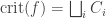$\mbox{crit}(f)=\bigsqcup_i C_i$ is a disjoint union of connected submanifolds $C_i$ , such that, if we denote by $\nu(C_i)$ the normal bundle of $C_i$ inside $M$ , then $Hess_p(f)\vert_{\nu(C_i)}$ is non-degenerate.

Loosely speaking, the degeneracies are “well-controlled”, and come in “families”. In general, in the Morse-Bott situation, one hopes for a perturbation scheme which recovers the non-degenerate/Morse case, by a small perturbation of the data, in such a way that one gets a 1-1 correspondence between the symmetric (i.e Morse-Bott) data, and the generic (i.e Morse) one, and so that compuations can be carried out in the Morse-Bott setting in the first place. For instance, if one wishes to compute Morse homology from a Morse-Bott function $f$ , one can choose a Morse function $h$ on $\mbox{crit}(f)$ , and consider $f_\epsilon:=f+\epsilon \rho h$ , for $\epsilon>0$ small, and $\rho$ is a bump function with support near $\mbox{crit}(f)$ . The critical points of $f_\epsilon$ are exactly those of $h$ , and there is a well-defined notion of convergence of flow-lines of $f_\epsilon$ to “cascades” (when the perturbation parameter $\epsilon$ is taken to go to zero). The latter consist of a flow-line of $f$ hitting a critical manifold, followed by a flow-line segment of $h$ along this manifold, followed by another flow-line of $f$ hitting another critical manifold, and so on, finishing in a critical point of $f$ (see the figure below). One can define the index of a cascade in such a way that the index is preserved under this convergence, and there is a 1-1 correspondence between index $I$ cascades and index $I$ Morse flow-lines of $f_\epsilon$ . Hence, one can define a Morse-Bott differential which counts cascades, and the resulting Morse-Bott (co)homology coincides with the usual Morse (co)homology.

drawing

In the setting of symplectic homology, if $W$ is a Liouville filling of a contact manifold $(M,\xi)$ and $H$ is an admissible autonomous Hamiltonian, then we have closed Hamiltonian orbits in the contact slices $\{r\}\times M$ corresponding to closed Reeb orbits, which come in $S^1$ -families obtained by reparametrizations (since $H$ is time-independent). This is then a Morse-Bott situation.

[Bourgeois-Oancea] In the Morse-Bott situation described above, if we assume that the orbits come in $S^1$ -families (and there are no further directions of degeneracy), then there is a Morse-Bott version of symplectic homology of $W$ , $SH_{MB}(W)$ .

More generally, one can ask the following Morse-Bott conditions: $\mathcal{N}_T:=\{m|\varphi^T(m)=m\}$ is closed submanifold (where $\varphi^T$ is the time $T$ Reeb flow), such that $rank(d\alpha\vert_{\mathcal{N}_T})$ is locally constant and $T\mathcal{N}_T=\ker(d\varphi^T-id)$ . Informally, one can think of this as an infinite-dimensional version of the Morse-Bott conditions, applied to the action functional defined on the loop space, whose critical points are closed Hamiltonian orbits. Assuming that $c_1(W)=0$ and the closed orbits are contractible (so we get an integer grading), fix a choice of Morse functions $f_T$ on $\mathcal{N}_T$ for every $T$ . The generators will correspond to pairs $(\gamma,T)$ where $\gamma \in \mbox{crit}(f_T)$ , and the differential counts “Floer cascades”, consisting of a Floer cylinder, followed by a flow-line segment of a $f_T$ , followed by another Floer cylinder…(finitely many times). The grading is defined by $|(\gamma,T)|=\mu_{RS}(\mathcal{N}_T)+ind_{\gamma}(f_T)-\frac{1}{2}(\dim(\mathcal{N}_T)-1)$ , where $\mu_{RS}$ is the Robin-Salamon index, and with this definition the differential has degree -1. Under these conditions, we have a Morse-Bott version of symplectic homology $SH_{MB}$ .

Uebele’s computation

We focus now on the Brieskorn manifolds $\Sigma_l^n:=\Sigma(2l,2,\dots,2)$ , where there are $n$ 2’s, for odd $n$ , endowed with the contact structure discussed in the first part of this talk. Randell’s algorithm gives $H_{n-1}(\Sigma_l^n)=\mathbb{Z}$ , and it follows from Wall’s classification of highly-connected manifolds that $\Sigma_l^n \simeq S^{n-1}\times S^n$ if $l\equiv 0 (mod 4)$ , $\Sigma_l^n \simeq S^*S^n$ if $l\equiv 1 (mod 4)$ , $\Sigma_l^n \simeq S^{n-1} \times S^n \# K$ if $l\equiv 2 (mod 4)$ , $\Sigma_l^n \simeq S^*S^n \#K$ if $l\equiv 3 (mod 4)$ . Here, $K=\Sigma(2,\dots,2,3)$ is Kervaire’s sphere. If $n=3$ , $K$ is diffeomorphic to $S^5$ , and hence $\Sigma_l^5$ is always $S^2 \times S^3$ .

These contact manifolds manifolds are actually not distinguishable by contact homology. However, we have:

Thm. [Uebele] The manifolds $\Sigma_l^n$ are pairwise non-contactomorphic.

This uses the following lemma:

Lemma. For $\Sigma_l^n$ , $SH_{MB}^+$ is independent of the filling, as long as $c_1(W)\vert_{\pi_2(W)}=0$ .

This is proved by showing that these manifolds are dynamically convex, and using an analogous version of Bourgeois-Oancea result. Therefore one can regard $SH_{MB}^+$ as a contact invariant.

The idea now is to compute $SH_{MB}^+$ of the natural filling of these Brieskorn manifolds, using the Morse-Bott techniques, and showing that they are pairwise different. One can choose perfect Morse functions along the critical manifolds (or “formally pretend” that one can, by a spectral sequence argument due to Fauck), making the Morse differential trivial, and between different critical manifolds, one sees that for each consecutive degrees $N, N+1$ there exists a unique pair of generators having these degrees, the one with bigger degree $N+1$ having lower action than the one with smaller degree $N$ . Since the differential has degree -1 and lowers the action, it has to vanish (this works for $n\geq 5$ , and a different argument is needed for $n=3$ ). The upshot is that the Morse-Bott symplectic homology coincides with its chain complex, and the degrees differ for different values of $l$ .

References

A nice reference for a survey of Brieskorn manifolds in contact topology can be found here: https://arxiv.org/abs/1310.0343

Ustilovsky’s exotic spheres: 1999-14-781

Uebele’s computations: https://arxiv.org/abs/1502.04547

Fauck’s thesis (related, and uses RFH): https://arxiv.org/abs/1605.07892

1 Comment

Filed under Uncategorized

by ksackel | July 9, 2017 · 10:17 pm

Kylerec – Weinstein fillings

Continuing on with the Kylerec posts… (see the first one here as well as notes to follow along with here).

This post is a synthesis of the following talks:

Day 1 Talk 2 – François-Simon Fauteux-Chapleau’s talk on Weinstein handles and contact surgery
Day 1 Talk 3 – Orsola Capovilla-Searle’s talk on Kirby calculus for Stein manifolds
Day 1 Talk 4 – Alvin Jin’s talk on Lefschetz fibrations and open books
Day 2 Talk 1 – Bahar Acu’s talk on mapping class factorizations and Lefschetz fibration fillings
Day 3 Talk 2 – Sarah McConnell’s talk on applications of Wendl’s theorem to fillings
Day 5 Talk 1 – Ziva Myer’s talk on flexible and loose Legendrians

Weinstein surgery theory

I assume the reader is familiar with smooth surgery theory. Recall the following definition.

Definition: A Weinstein cobordism consists of a quadruple $(W,\omega,V,\phi)$ , where

$(W,\omega)$ is a compact symplectic manifold with boundary
$V$ is a Liouville vector field for $(W,\omega)$ , meaning $\mathcal{L}_V\omega = \omega$ , which is also transverse to the boundary $\partial W$
$\phi \colon W \rightarrow \mathbb{R}$ is a Morse function
$V$ is gradient-like for $\phi$ , meaning there is some constant $\delta$ with $d\phi(V) \geq \delta(|d\phi|^2 + |V|^2)$ with respect to a given Riemannian metric.

In this case, the boundary decomposes as $\partial W = \partial^+ W \sqcup \partial^-W$ , where $V$ points out of $\partial^+ W$ and into $\partial^- W$ . Note that the 1-form $\lambda = \iota_V \omega$ satisfies $d\lambda = \omega$ , and is sometimes called the Liouville 1-form, since it encodes the same data as $V$ . Also note that a Weinstein cobordism with $\partial^- W = \emptyset$ is what we called a Weinstein filling.

The gradient-like condition is meant to give $V$ some directionality (since $d\phi(V) > 0$ ) and ensure that the critical points of $V$ are non-degenerate. One typically doesn’t think of the precise choice of pair $(V,\phi)$ as very important, but rather the data up to some notion of homotopy. For example, one can always perturb the Morse function so that each of $\partial^- W$ and $\partial^+ W$ is a regular $\phi$ -level set, regardless of the number of components, and so we might as well assume this from the start. The equivalence hinted at here is called Weinstein homotopy, by which we perturb the pair $(V,\phi)$ , possibly through birth-death type singularities.

Lemma: The descending manifolds in a Weinstein cobordism, i.e. the set of points which flow along $V$ to a given critical point in infinite time, are isotropic submanifolds.

Proof: Standard Morse theory implies these submanifolds are smooth. Let $\phi_V^t$ be the flow along $V$ at time $t$ , and suppose we choose some $q \in D_p^-$ where $D_p^-$ is some descending manifold for a given critical point $p$ . Suppose $v \in T_qD_p^-$ is a vector in the tangent space. Then since $\mathcal{L}_V\lambda = d\iota_V\lambda + \iota_V d\lambda = d\iota_V^2\omega + \iota_V\omega = 0 + \lambda = \lambda$ , we have that

$e^t\lambda_q(v) = ((\phi_V^t)^*\lambda)(v) = \lambda(d\phi_V^t(v))$

As $t \rightarrow \infty$ , the right hand side goes to zero since $\phi_V^t(q') \rightarrow p$ for all $q'$ in a curve $\gamma$ along $D_p^-$ with tangent vector $v$ at $q$ . Hence, $\lim_{t\rightarrow \infty} e^t \lambda_q(v) = 0$ , from which it follows that $\lambda_q(v) = 0$ . Hence, $\lambda|_{D_p^-} = 0$ , and so also $\omega|_{D_p^-} = d\lambda_{D_p^-} = 0$ .

Corollary: All critical points in a Weinstein cobordism $(W^{2n},\omega,V,\phi)$ are of index at most $n$ . Smoothly, any such manifold can be built up by surgery starting from a neighborhood of $\partial^-W$ and attaching handles of index at most $n$ .

One would like to be a bit more precise about how the surgery interacts with the symplectic geometry. As a first step, along a regular level set $W_c := \phi^{-1}(c)$ , the symplectic condition on $\omega$ implies that $\lambda|_{W_c}$ is a contact form. The proof of the lemma above further implies that $D_p^- \cap W_c$ gives an isotropic submanifold of $W_c$ with respect to $\lambda|_{W_c}$ .

So we can think, at least smoothly, that our Weinstein cobordism is built up, starting from $\partial^- W$ , by attaching handles with isotropic cores and attaching spheres along isotropics in level sets of $\phi$ (which are contact submanifolds). But there’s a little more that we know about neighborhoods of isotropics. In a symplectic manifold, the neighborhood of an isotropic $M \subset (W,\omega)$ is completely determined up to symplectomorphism by its symplectic normal bundle, $(TM)^{\omega}/TM$ , as a symplectic vector bundle (with symplectic structure induced by $\omega$ on the fibers). A similar statement holds for isotropic submanifolds in contact manifolds, but now with their neighborhoods determined up to contactomorphism by the conformal symplectic normal bundle $(TM)^{d\alpha}/TM$ , where $\alpha$ is a contact form so that $d\alpha$ is symplectic on $\xi$ . Furthermore, if we fix $\alpha$ , then the symplectic vector bundle structure determined by $d\alpha$ on the nose determines the neighborhood up to exact contactomorphism. Patching these two things together, one finds:

Theorem [Weinstein, before the term “Weinstein handle” was coined]: Weinstein handle attachment is completely specified (up to Weinstein homotopy) by matching the symplectic framing data determined by $\lambda$ along the isotropic attaching spheres.

One therefore thinks of $\partial^+ W$ as being built up from $\partial^- W$ by contact surgery along isotropic submanifolds with given framing information compatible with the underlying symplectic topology.

Consider a Weinstein cobordism of dimension $2n$ . Then the handles of index $k \in \{0,1,\ldots,n-1\}$ are called subcritical handles, whereas the handles of index $k = n$ are called critical handles. When $k = n$ , the aformenetioned symplectic normal bundles are trivial automatically, and so one specifies critical handle attachment simply by drawing a Legendrian sphere on $\partial^- W$ .

Recall that the proof of the h-cobordism theorem requires some ability to cancel (and create) pairs of handles with index differing by 1 whose ascending and descending manifolds intersect in a 1-dimensional manifold, to move around attaching spheres, and to move critical values around. The last of these we can always do, so we can attach the handles in order of their index. It turns out that when $2n > 4$ , we can recreate all parts of the proof of the h-cobordism theorem for subcritical Weinstein cobordisms. In some sense, subcritical Weinstein domains have no symplectic geometry in them – they are encoded by algebro-topological information, and so this gives some flexibility phenomena.

It turns out that some critical handles behave the same way. The key obstruction to the aforementioned flexibility is that sometimes the data of an attaching Legendrian does not boil down to purely toplogical information. However, Emmy Murphy defined a class of Legendrians, called loose Legendrians, for which there is such a so-called h-principle. The Weinstein h-cobordism theorem works for Weinstein cobordisms which can be built (up to Weinstein homotopy) out of subcritical and loose critical handle attachments. We call such Weinstein cobordisms flexible.

We often care about the case when $2n = 4$ . In this case, it is pretty easy to describe a connected Weinstein domain (or its contact boundary). One can first order the handles by index, and then cancel 0-handles with 1-handles until we are in the situation where there is precisely one 0-handle and possibly many 1- and 2-handles. The boundary of the 0-handle is just a standard contact $S^3$ , and 1-handle attachment is trivially described by picking pairs of points in $S^3$ (the bundle data boils down to showing $\pi_0(\text{Sp}(2,\mathbb{R})) = 0$ ). So it suffices to draw Legendrians on $S^3$ with $k$ pairs of points identified, which is just $\#^k (S^1 \times S^2)$ . 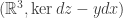Any Legendrian $L$ has a canonical framing of its normal bundle given by the twisting of the Reeb chord around the Legendrian. Eliashberg showed that adding a left twist to this framing gives the smooth framing which determines the corresponding smooth surgery data.

Gompf showed that in this case $2n = 4$ , one can draw standard Kirby calculus type surgery diagrams. We think of all of these 1-handle attachments and Legendrians as missing a point in $S^3$ , so that we can draw our diagrams in $(\mathbb{R}^3, \ker dz - ydx)$ . The front projection is the projection to the coordinates $(x,z)$ , so that $y$ is determined by $dz/dx$ . It might not be obvious how to draw a smooth knot in this projection since the curve can’t have infinite slope, but we are allowed semi-cubical cusps, corresponding to 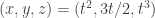$(x,y,z) = (t^2,3t/2,t^3)$ . Note that transverse crossings are also allowed, since the $y$ -coordinates are distinct. One usually draws the front projection of a Legendrian without showing which strand lies over the other, but we include this extra information in the next figure, where we imagine the $y$ -axis as pointing into the page.

A Legendrian trefoil knot

Gompf’s standard form for these Legendrians looks like the following, where the pairs of balls in each row corresponds to where the 1-handles are attached, and the Legendrian strands simply go through the handles as though they were wormholes.

An example of a Gompf surgery diagram. There are three 1-handles (in blue, red, and green) and two 2-handles with attaching spheres given by the Legendrian tangle above. All of the information can be made to live inside of the purple rectangle (i.e. without going horizontally or vertically outside of where the 1-handles are attached).

Weinstein fillings, Lefschetz fibrations, and open book decompositions

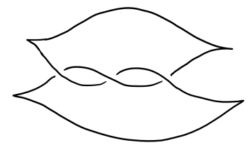
Definition: A Lefschetz fibration is a smooth map $\pi \colon W^4 \rightarrow \Sigma^2$ with finitely many critical points with distinct critical values such that locally around the critical points, $\pi$ looks like a complex Morse function (i.e. $(z_1,z_2) \mapsto z_1^2+ z_2^2$ in local coordinates). When $\Sigma$ has boundary, we assume the critical values of $\pi$ are all in the interior of $\Sigma$ .

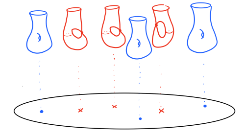
We shall typically be concerned with the case where $\Sigma = \mathbb{D}$ (although see this post by Laura Starkston which slightly generalizes some of what is discussed here).

A schematic for a Lefschetz fibration over the disk

In the case where $\Sigma = \mathbb{D}$ , we see that the boundary decomposes as $\partial W = \partial^v W \cup \partial^h W$ , where the superscripts are meant to indicate vertical and horizontal. That is, $\partial^v W = \pi^{-1}(\partial \mathbb{D})$ , while $\partial^hW = \sqcup_{p \in \mathbb{D}} \partial \pi^{-1}(p)$ . If we write $F$ for a regular fiber of $\pi$ , then $\partial^h W = \partial F \times \mathbb{D}$ . 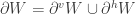Meanwhile, we see that $\partial^v W$ is just a fibration over $S^1$ with fiber $F$ , and hence can be described by some monodromy map $\phi \colon F \rightarrow F$ fixing the boundary, so that $\partial^v W = F \times [0,1]/{\sim}$ where $(\phi(x),0) \sim (x,1)$ (the mapping torus of $\phi$ ).

The structure on the boundary, in which we have a fibration over $S^1$ with fiber $F$ glued together with $\partial F \times \mathbb{D}$ in the natural way, is called an open book decomposition. It is given completely by the pair $(F,\phi)$ . We think of each fiber over $S^1$ as a page, and the subset $F \times \{0\}$ as the binding, analogous to what one would get if one took their favorite book and matched the covers so that the pages radiate outwards. So Lefschetz fibrations yield open books on the boundary. To be a little more precise, one should extend each page so that the boundary of each page is actually the binding.

Some pages near the binding of an open book. I guess the name “Rolodex” wasn’t as catchy as “open book.” (Image from Wikipedia)

Now suppose $0 \in \mathbb{D}$ is a regular value (which can always be arranged up to small perturbation of $\pi$ ). Then $\pi^{-1}(\epsilon \mathbb{D}) \cong F \times \mathbb{D}$ . One can ask what happens when we extend to $\pi^{-1}(U)$ , where $\epsilon \mathbb{D} \subset U$ and there is exactly one critical value $p$ on $U \setminus \epsilon\mathbb{D}$ .

Since we have a nice fibration away from critical points, we see that paths in $\mathbb{D}$ yield monodromy maps (up to isotopy preserving boundary) on the fibers. We can choose a connection on the fibration if we wish to make this a map on fibers, not just a map up to isotopy. 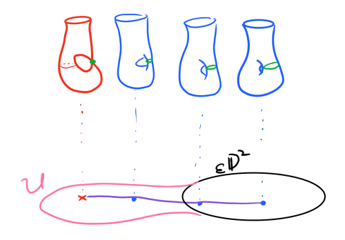If we take a path $\gamma$ from 0 to $p$ which intersects $\partial \epsilon \mathbb{D}$ once and otherwise avoids critical values then for whatever connection we chose, we can see what points flow to the critical point over $p$ . Over each regular fiber, this is just a circle, and the union of all of them together with the critical point yields a disk. The path $\gamma$ is called a vanishing path, and each circle on the regular fiber is called a vanishing cycle (one really should think of it as a homology cycle, but for concreteness, one can think of it as a curve). The disk consisting of the union of vanishing cycles above a path is called a thimble.

The green circles in the regular fibers above the purple vanishing path are the vanishing cycles. Their union is the thimble.

It is then not hard to see that $\pi^{-1}(U)$ is obtained from $\pi^{-1}(\epsilon \mathbb{D})$ by 2-handle attachment, where the attaching curve is just the vanishing cycle above $\gamma \cap \partial \epsilon \mathbb{D}$ and the core of the handle is the thimble. Furthermore, one can check by a local computation that the monodromy map in a loop around $p$ is just given by a Dehn twist (positive or negative, depending on orientations) around the vanishing cycle. Hence, one can write out the open book determined by the Lefschetz fibration explicitly – it is just the product of the Dehn twists on the vanishing cycles, performed in an order determined by a sequence of vanishing paths.

Notice that for a given regular value on $\partial \mathbb{D}$ , one can choose a different basis of vanishing paths, and this yields a possibly different factorization for the monodromy. Such changing of the basis is generated by so-called Hurwitz moves, as drawn below.

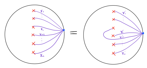
A Hurwitz move swapping the $i$ th and $(i+1)$ st critical points. Note that the corresponding vanishing cycles for the critical point corresponding to $\gamma_i$ and $\gamma_{i+1}'$ are actually different, but the overall monodromy on the open book at the boundary is the same.

Hence, understanding Lefschetz fibrations over the disk essentially corresponds to understanding factorizations of mapping class group elements into Dehn twists.

Now, this whole story can be repeated in the symplectic context, as follows.

Definition: A symplectic Lefschetz fibration is a Lefschetz fibration with $(W,\omega)$ a symplectic manifold such that each fiber is symplectic submanifold away from the critical points, while at the critical points the coordinates in which $\pi$ locally looks like a complex Morse function can be taken to be holomorphic for some compatible almost complex structure $J$ .

In this case, one can take the connection to be the symplectic connection given the symplectic orthogonal complement to the vertical directions. In this way, the thimbles produced will actually be Lagrangian disks, which suggests one can think of these as the descending disks for a Weinstein domain filling the boundary. In addition, the monodromy maps are now compositions of positive Dehn twists only, since the symplectic condition gives the proper orientations. In other words, our Lefschetz fibration is itself positive. If the vanishing cycles of a Lefschetz fibration are homologically nontrivial, we shall call it allowable.

With a little more work, we can obtain the following theorem of Loi and Piergallini (although an alternative proof by Akbulut and Özbağci is more in line with the exposition presented here):

Theorem: Any positive allowable Lefschetz fibration (PALF) yields a Weinstein domain, and any Weinstein domain comes from a PALF in this way.

Furthermore, one obtains a little bit more compatibility at the boundary.

Definition: An open book decomposition on a manifold $M$ is said to support a cooriented contact structure $\xi$ if there is some contact form $\alpha$ for $\xi$ such that the binding is a contact submanifold, $d\alpha$ is a symplectic form on the pages, and the boundary orientation of the page (with respect to $d\alpha$ ) matches the orientation of the binding with respect to $\alpha$ .

One checks that the open book on the boundary of a PALF does indeed support the contact structure determined by being the boundary of a Weinstein domain.

Our surgery theory for these Lefschetz fibration builds the fiber up by subcritical surgery, and the 2-handle attachments correspond to the critical points of the fibration. One can always produce, for any Weinstein manifold, a cancelling pair consisting of a 1-handle and a 2-handle. The way that this affects the open book is by positive stabilization, meaning that one adds a 1-handle to the page, but kills it by adding an extra Dehn twist to the monodromy through a circle which passes through the handle.

The following theorem implies that all 3-dimensional contact geometry can actually be encoded (somewhat non-trivially) in the study of open books up to positive stabilization, and hence the study of Weinstein fillings reduces to studying positive factorizations of given elements of the mapping class group of a surface with boundary (up to this not-so-easy-to-work-with notion of positive stabilization).

Theorem [Giroux correspondence]: There is a one-to-one correspondence between contact structures on a closed 3-manifold up to isotopy with open books up to positive stabilization.

Applications to Weinstein fillings

To summarize the previous section, an explicit surgery decomposition of a Weinstein filling yields a PALF which in turn gives an open book structure supporting the contact boundary of the Weinstein filling with monodromy factored into positive Dehn twists. Conversely, given a supporting open book for a contact structure with monodromy factored into positive Dehn twists, one obtains a Weinstein filling.

One common question we ask is whether a single contact manifold has multiple Weinstein fillings. From the above construction, one possible way to attack this problem is to look for distinct positive factorizations of a given element in a mapping class group.

Theorem [Auroux]: There is an element in the mapping class group of the surface $\Sigma_{1,1}$ (of genus 1 and with one boundary component) with two distinct factorizations into positive Dehn twists such that the Weinstein fillings are distinguished by their first homology.

Remark: In this setting, the first homology is just given by $H_1(F)/V$ where $V$ is the span of the vanishing cycles. The only real trick of Auroux is therefore to find a good candidate for the above theorem to hold, and just compute.

Generalizing a bit more:

Theorem [Baykur – Van Horn-Morris]: There exists an element in the mapping class group of $\Sigma_{1,3}$ (of genus 1 with three boundary components) which admits infinitely many positive factorizations such that the corresponding Weinstein fillings are all distinguished from each other by their first homology.

Finally, as one last application, I want to consider a result of Plamenvskaya and Van Horn-Morris, but I need to define the contact structures in question to begin. Honda’s classification of tight contact structures on the lens spaces $L(p,1)$ can be formulated in Gompf’s surgery diagrams by the following diagrams, coming from a single 2-handle attachment to standard $S^3$ . We denote the corresponding contact structures by $\xi_1,\xi_2,\ldots, \xi_{p-2}$ .

The surgery diagram for the contact structure $\xi_k$ .

Of these, the universal covers of $\xi_1$ and $\xi_{p-2}$ are also tight, where as the others’ universal covers are overtwisted. We say $\xi_2, \ldots, \xi_{p-3}$ are virtually overtwisted.

Theorem [PV]: Each virtually overtwisted $(L(p,1), \xi_k)$ has a unique Weinstein filling (up to symplectic deformation) and a unique minimal weak filling.

Proof sketch: Let us first discuss the Weinstein part. There are a few nontrivial theorems which go into this, which we won’t discuss, but essentially we have the following sequence of results. The open book given by the surgery diagrams above induce open books with genus 0 pages. When we discussed Wendl’s theorem in part 2 of the J-holomorphic curve posts, one thing we mentioned was that one can apply his techniques when there is a planar open book (meaning pages have genus 0). He proves that if a contact manifold has a given supporting planar open book, then every Weinstein filling is diffeomorphic to one compatible with that specified planar open book. Hence, it suffices to study Lefschetz fibrations compatible with the one just described, which in turn becomes studying factorizations of an element in the mapping class group of $\mathbb{D}_n$ , the disk with $n$ holes. A nontrivial result of Margalit and McCammond gives that every such presentation must be in a certain form, from which one can use smooth Kirby calculus to conclude that the surgery diagram must come from $-p$ -surgery on some knot. Finally, an appeal to work of Kronheimer, Mrowka, Ozsváth, and Szabó using Seiberg-Witten Floer homology (also called monopole Floer homology) yields that this knot must have been an unknot, and since the framing is $-p$ , this determines the canonical framing of the knot, which in turn implies we could only have had one of our original surgery diagrams.

Finally, to obtain the weak part, one can use work of Ohta and Ono to boost a weak filling up to a strong filling, from which Wendl’s theorem implies that any minimal weak filling is symplectic deformation equivalent to a Weinstein filling.