Category Archives: Conference Notes

by AHM | August 9, 2012 · 6:59 pm

Lattice Homology and Knots

I’m excited to be joining the blog. I’ve been consumed mainly by watching talks and meeting people at the Stanford conference, so this first post will consist only of my notes from Andras Stipsicz‘s talk on lattice homology. The content of the talk represents joint work of Stipsicz with Ozsváth and Szabó. I don’t have a lot of experience with lattice homology, so if I’ve missed or misunderstood something, please contribute your corrections in the comments section.

The talk began with a review of the standard Heegaard Floer package. Knot Floer homology was recently mentioned on the blog when Laura discussed Zoltan Szabó’s research talk at Budapest. So, if you’d like a refresher on notation, please check out that post (but feel free to skip the bordered part if you’re in a rush).

With an powerful invariant like Heegaard Floer (or knot Heggaard Floer), a lot of people are interested in how to compute it. Stipsicz gave an overview of some of the pertinent questions about computation and existing technology.

Computational aspects:

How to compute the invariant in a simple way?
How to prove invariance in a simple way? (Simple here means without infinite dimensional analysis or having to count pseduoholomorphic curves.)
Can you find an effective way of computing invariants? (Effective depends on your personal opinion of an efficient algorithm.)

Existing technology:

Sarkar-Wang (2006) – “Nice” diagrams allow you to compute HF-hat.
Manolescu-Ozsváth-Sarkar and Manolescu-Ozsváth-Szabó -Thurston – Grid diagrams allow for a combinatorial descriptions of the knot and link invariants.
Ozsváth-Sarkar-Szabó (2007) – Verification of independence with special nice diagrams for HF.
New algorithms coming from Lipshitz-Ozsváth-Thurston’s bordered Floer homology.

The first two references mentioned are examples of simple ways to compute the invariants. The cost of theoretical simplicity, though, is a miserably inefficient algorithm. For example, the algorithm that computes HFK from a grid diagram has order of complexity somewhere in the neighborhood of $O(n^2!)$ . Yikes! The bordered techniques are computationally better, but require some rather difficult algebra.

So keeping these motivating issues in mind, let’s see what Stipsicz said about lattice homology and how it relates to Heegaard Floer.

Lattice homology
Suppose that $G$ is a tree with integer weights $m_i$ associated to its vertices $v\in V(G)$ . We consider the plumbing construction $G \rightsquigarrow X_G$ . This means that $X_G$ is the compact oriented 4-manifold obtained by plumbing $D^2$ bundles over $S^2$ with Euler numbers given by the weights $m_i$ and plumbing instructions indicated by the graph. The three dimensional boundary $Y_G = \partial X_G$ of the resulting manifold is our object of interest.

The construction that follows is due to Nèmethi in 2008:

Define $Char(G)$ to be $\{K:V\rightarrow \mathbb{Z} | K(v)=m_v$ mod 2 for all $v\}$ , i.e. the set of characteristic elements in the second integral cohomology group of $X_G$ .

Let $\mathbb{CF}^-(G)$ denote the $\mathbb{Z}_2[U]$ module freely generated over $\mathbb{Z}_2[U]$ by pairs $[K, E]$ , where $K$ is a characteristic covector and $E$ is a subset of vertices in $V$ .
The differential of this complex is given by:

$\partial^-[K,E] = \Sigma_{v\in E} U^{a_v[K,E]} [K,E-v] + U^{b_v[K,E]} [K+2v^*,E-v]$

Those exponents $a_v$ and $b_v$ are integers which are defined with an auxiliary function $\mathcal{I}$ . If $I\subset E$ , then $\mathcal{I}[K,I] = \frac{1}{2}(\sum_{u\in I}K(u) + (\sum_{u\in I}u)^2 )$ . That second term represents a self-intersection in $X_G$ . Let:

$A_v[K,E] = \min\{ \mathcal{I} | I\subset E-v\}$
$B_v[K,E] = \min\{ \mathcal{I} | v\in I\subset E\}$
$a_v = A_v- \min \{A_v, B_v\}$
$b_v = B_v - \min \{ A_v, B_v \}$

Also note that since $K$ specifies a spin-c structure on $X_G$ , we associate to $K$ the spin-c structure $\mathfrak{s}_K \in Spin^c(Y_G)$ .

OK. That sets up the lattice homology, more or less. I don’t really understand what the differential is actually doing, but its apparent benefit is that it is defined in a combinatorial manner (i.e. no counts of holomorphic curves). If anyone would like to really understand this, it would probably be best to check out the papers by Nèmethi and Ozsváth, Stipsicz, and Szabó.

Rational graphs
My notes became somewhat illegible at this point in the lecture, so I’ve attempted to vet this section with some information from this paper. Let’s assume that $G$ is a negative definite plumbing graph. We’d like to get a handle on when $G$ is rational, and as it turns out, there is a combinatorial algorithm that does this.

Algorithm. Let $K_1 = \Sigma_{v\in V} v$ , and compute all of the products $K_1\cdot v$ . If:

any of the products is greater than or equal to 2, stop. $G$ is not rational.

all of the products are less than or equal to 0, stop. $G$ is rational.

any product $K_1\cdot v = 1$ , then set $K_2 = K_1+ v$ and repeat.

(I’m being a bit sloppy here with the notation; $v$ stands for both a vertex and the second homology class in the plumbed manifold corresponding to that vertex.) This algorithm produces a series of vectors $K_1, K_2, \cdots$ , and terminates in finite time. The product, by the way, is a dot product computed in the intersection matrix of the four-manifold. I believe $E_8$ was a suggested example of a rational graph on which to perform the algorithm.

Additionally, we say that $G$ is of type-k if there exists vertices $v_1, \cdots, v_k$ such that sufficiently decreasing the weights $m_{v_1}, \cdots m{v_k}$ makes $G'$ rational.

So why do we care about types of rational graphs? The following theorem of Nèmethi in 2008:
Theorem. Suppose $G$ is negative definite plumbing tree. Then,

$H_*( \mathbb{CF}^-(G, \mathfrak{s}), \partial^-) =\mathbb{HF}^-(G, \mathfrak{s})$ is a three-manifold invariant.
$G$ is rational if and only if $\mathbb{HF}^-(G, \mathfrak{s}) \cong \mathbb{Z}_2[U]$ for all spin-c structures over $Y_G$ .
If $G$ is of type-1 this implies $\mathbb{HF}^-(G, \mathfrak{s}) \cong HF^-(Y_G, \mathfrak{s})$ .

Moreover, there exists a surgery exact sequence for lattice homology, a result also obtained independently by Josh Greene. The theorem leads to the conjecture that $\mathbb{HF}^-(G, \mathfrak{s}) \cong HF^-(Y_G, \mathfrak{s})$ for any plumbing tree $G$ . To this end, there is a theorem of Ozsváth, Stipsicz, and Szabó that tells us there is a spectral sequence on $\mathbb{HF}^-(G, \mathfrak{s})$ converging to $HF^-(Y_G, \mathfrak{s})$ . If $G$ is of type-2, the spectral sequence collapses and the homology groups are isomorphic.

Refinement to knots

Are you still hanging in there? Great! Onward to knots.

Now, we let $\Gamma_{v_0}$ denote a plumbing graph with a distinguished, unweighted vertex $v_0$ . Define the lattice chain complex on $G=\Gamma_{v_0}-v_0$ . The vertex $v_0$ induces a filtration $\mathcal{A}$ on the lattice homology complex. For a generator $[K, E]$ of the lattice complex, the filtration level $\mathcal{A}[K,E]$ is given by a formula that is essentially the same as the auxiliary function $\mathcal{I}$ above, except it use a specific extension of $K$ and $E$ to $\Gamma_{v_0}$ . The filtered complex $(\mathbb{CF}^-(G, \mathfrak{s}), \partial^-, \mathcal{A}_{v_0})$ is the subject of the main theorem:

Theorem. Suppose the tree $\Gamma_{v_0}$ with distinguished vertex $v_0$ is given, that $G=\Gamma_{v_0}-v_0$ negative definite, and that $G_{v_0}(k)$ is negative definite* for $k\in \mathbb{Z}$ . Then $\mathbb{CF}^-(G, \partial^-, \mathcal{A}_{v_0})$ determines the lattice chain complex $\mathbb{CF}^-(G_{v_0}(k), \partial^-).$

(*I took $G_{v_0}(k)$ to mean that we’ve put a framing of $k$ on the vertex $v_0$ , large enough to ensure that $Y_{G_{v_0}}$ is an L-space.)

You might be asking yourself where does the knot fit into this picture? Well, when you do the plumbing, the unknot living at the distinguished vertex becomes knotted. That’s the knot. It’s also important to note that while knot Floer homology is defined for all knots, the construction described above is not. It works for connected sums of iterated torus knots, but certainly not all knots.

I do not have very detailed notes about the proof of the theorem, but it seemed to me to be a consequence of a complicated and formal similarity of homological algebra. In Heegaard Floer, $CF^\infty$ is a doubly filtered complex. The filtrations can be used to chop up the complex into various subcomplexes, and then these these subcomplexes, the maps relating them, and their mapping cones are used to describe the Heegard Floer of surgeries along $K$ . Here is a paper that details this construction.

Apparently, lattice homology also enjoys such a structure. The ‘infinity’ lattice complex $\mathbb{CF}^\infty(G) = \mathbb{CF}^-(G)\otimes_{\mathbb{Z}_2} \mathbb{Z}_2[U^{-1}, U]$ is doubly filtered by the action of $U$ and an extension of $\mathcal{A}$ . It, too, can be chopped up into subcomplexes, the mapping cones of which are quasi-isomorphic to lattice complexes of $G_{v_0}(k)$ .

Relating the Heegaard Floer and lattice complexes takes more work. Unfortunately, there isn’t much I am able to say about this. So, let me just say that lattice homology is really interesting and I’m looking forward to learning more about it.

I’ll sign-off by reporting the big result in Ozsváth, Stipsicz, and Szabó‘s paper.
Theorem. If $G$ is a plumbing graph with a distinguished vertex $v$ such that the components of $G-v$ are all rational, then the filtered chain complex of $\Gamma_{v_0}$ in lattice homology is filtered chain homotopy equivalent to the filtered complex for $Y_G$ in Heegaard Floer.

…and it’s wonderful corollary:
Corollary. The lattice homology of a knot in $S^3$ is equal to its knot Floer homology.

1 Comment

Filed under Conference Notes

Tagged as 3-manifolds, Heegaard Floer, knots, lattice homology

by lstarkston | August 8, 2012 · 11:30 pm

Concordance

There are a lot of research talks this week at Stanford, so I’ll write about a few of them in the next few days.

Matt Hedden and Jen Hom both gave talks about knot concordance, so I’ll talk about what both of them said here. One goal in studying knot concordance is to try to understand something about 4-manifolds. Finding knots with certain concordance properties can be used to show the existence of exotic $\mathbb{R}^4$ ‘s. While knot concordance may not be able to tell us everything about smooth 4-manifolds, it can lead to interesting results. The goal then is to learn as much as possible about the size and structure of the concordance group.

Concordance definitions:

Two knots are smoothly concordant if they are the boundary of a proper embedding $(S^1\times[0,1], S^1\times\{0,1\})\to (S^3\times[0,1], S^3\times\{0,1\})$ . This is an equivalence relation, and the space of knots modulo concordance equivalence forms an abelian group, (addition is connected sum, the unknot is the identity, and negation is the mirror image with reversed orientation). An equivalent definition for $K_1$ and $K_2$ to be concordant is that $K_1\#\overline{K_2}^r$ is smoothly slice (bounds a disk in the 4-ball). We can also consider the topological concordance equivalence, which instead of requiring the above mapping of the cylinder to be smooth, we only require that it is continuous and extends to a continuous map on a tubular neighborhood. Topological concordance is a weaker equivalence than smooth concordance. Let $\mathcal{C}$ denote the group of knots up to smooth concordance, and $\mathcal{C}^{top}$ denote the group of knots up to topological concordance.

There is good motivation to focus on topologically slice knots (topologically concordant to the unknot), up to the equivalence relation given by smooth concordance. Denote this space by $\mathcal{C}_{TS}$ . Showing that $\mathcal{C}_{TS}$ is non-trivial implies the existence of exotic $\mathbb{R}^4$ ‘s.

History of results regarding $latex\mathcal{C}_{TS}$:

Casson showed in 82 using Donaldson’s diagonalization theorem that there are knots with trivial Alexander polynomial, which are not smoothly slice. Freedman showed around the same time that knots with trivial Alexander polynomial are necessarily topologically slice. Combining these results shows that $\mathcal{C}_{TS}$ is non-trivial.

In 95 Endo showed that this group is big, namely there is a copy of $\mathbb{Z}^{\infty}\subset \mathcal{C}_{TS}$ . Livingston, and Manolescu-Owens more recently showed that $\mathcal{C}_{TS}$ contains a direct summand of $\mathbb{Z}^3$ distinguished using the $\tau$ and $s$ invariants from Heegaard Floer and Khovanov homologies, which are both concordance invariants.

Satellite operations and concordance:

One operation on knots that works compatibly with concordance is forming satellites. Given a pattern knot P embedded in a solid torus, one obtains a map from knots to knots sending a knot K, to its satellite with that pattern P(K) (embed the pattern solid torus in a neighborhood of the knot K). A particularly useful example is the Whitehead double whose pattern is:

It is a consequence of the Skein relation that the Whitehead double of a knot is trivial (resolve the crossing at the clasp), so by Freedman’s result above, all Whitehead doubles are topologically slice, and thus represent elements of $\mathcal{C}_{TS}$ . One may want to understand how many elements in $\mathcal{C}_{TS}$ can be represented by Whitehead doubles. Hedden and Kirk prove that there there is a $\mathbb{Z}^{\infty}\subset Image(D) \subset \mathcal{C}_{TS}$ . The knots are Whitehead doubles of torus knots, and the proof uses SO(3) gauge theory to show the knots are not smoothly concordant.

Another infinite family of independent topologically slice knots formed via satellite operations, which is independent of both Endo’s examples and the above examples, are (p,1) cables of the Whitehead double of the right-handed trefoil. Jen Hom distinguishes these in the concordance group using her concordance invariants from Heegaard Floer homology. She defines an invariant $\varepsilon\in \{-1,0,1\}$ which can be computed from the chain complex $CFK^{\infty}(K)$ through an algebraic process involving the $\tau$ invariant (which is also a concordance invariant), or more geometrically by looking at the triviality or nontriviality of cobordism maps on $\widehat{HF}$ induced by large integer surgeries on the knot in $S^3$ . This is a concordance invariant of the knot, and it can be used to create a new equivalence relation on knots through their Heegaard Floer chain complexes. The idea is as follows. We can associate to a knot K, the complex $CFK^{\infty}(K)$ and to its inverse in the concordance class, we get $(CFK^{\infty}(K))^*$ . The analog of addition in the knot concordance group is the tensor product of chain complexes by the following Kunneth formula: $CFK^{\infty}(K_1\#K_2) = CFK^{\infty}(K_1)\otimes CFK^{\infty}(K_2)$ . If a knot K is smoothly slice, then $\varepsilon(CFK^{\infty}(K))=0$ . With the concordance equivalence relation, we started with a monoid of knots under connected sum, and mod out by the concordance equivalence relation to get a group. Similarly, the $CFK^{\infty}$ complexes form a monoid under tensor product and we obtain a group if we mod out by the equivalence relation $CFK^{\infty}(K_1)\sim_{\varepsilon} CFK^{\infty}(K_2) \iff \varepsilon(CFK^{\infty}(K_1)\otimes CFK^{\infty}(K_2)^* = 0$ . The resulting group $\mathcal{F} = \{CFK^{\infty}(K): K\subset S^3\}/\sim_{\varepsilon}$ has additional useful structure: a total ordering, a notion of much greater than, and a filtration. These structures can be used to show linear independence of knots in the concordance group.

Based on how $\varepsilon$ is defined, there is definitely a relation to the $\tau$ invariant, but $\varepsilon$ is a more powerful invariant. It turns out that the exact relation is related to the satellite operation. Jen proved that $CFK^{\infty}(K_1)\sim_{\varepsilon} CFK^{\infty}(K_2)$ if and only if $\tau(P(K_1)) = \tau(P(K_2))$ for every pattern P. Furthermore the satellite map descends to a well defined map on the group of knots up to $\varepsilon$ equivalence.

More pieces of the topologically slice concordance group:

Since we have a lot of examples of independent concordance classes with trivial Alexander polynomial obtained by Whitehead doubles, one may ask whether the smallest subgroup generated by knots with trivial Alexander polynomial gives all topologically slice concordance classes, i.e. does $\mathcal{C}_{\Delta} := \langle \{[K]: \Delta_K=1\}\rangle = \mathcal{C}_{TS}$ ? The answer to this question is strongly no. Hedden and Livingston prove that there is an infinitely generated free abelian subgroup in the quotient: $\mathbb{Z}^{\infty}\subset \mathcal{C}_{TS}/\mathcal{C}_{\Delta}$ .

So now we know that there are lots of knot concordance classes with trivial Alexander polynomial, lots with nontrivial Alexander polynomial, but each of these constructions produce concordance classes of infinite order. We can also ask about torsion in the knot concordance group. The easiest kind of torsion to understand is 2-torsion. In this case $0=2[K]$ so $[K]=-[K]=[\overline{K}^r]$ , i.e. the knot is isotopic to its reverse mirror image. Such knots have been studied for awhile, and are called amphichiral. There are lots of such knots, so it is reasonable to expect some of the topologically slice knots to have this property.

Indeed there are lots of amphichiral knots which are smoothly concordance independent, but also topologically slice. The theorem is due to Hedden, S.G. Kim, and Livingston:
$(\mathbb{Z}/2)^{\infty} \subset \mathcal{C}_{TS}$ .

The knots is this family are constructed by starting with an amphichiral knot that is not topologically slice, and then performing satellite operations with different knots, and taking connected sums to obtain topologically slice knots that are amphichiral. Next one needs to show that these knots are not smoothly slice, and that they represent independent concordance classes. Here you need Heegaard Floer homology. The obstruction to K being slice comes from the d-invariant. The d-invariant, $d(Y,\mathfrak{s})$ is keeping track of the highest grading of the generator of the nontorsion elements in the (minus) Heegaard Floer homology of a $\mathbb{Z}/2$ homology 3-sphere. To use this to obstruct sliceness, first one notices that if K were smoothly slice, then its branched double cover $\Sigma(K)$ would be a $\mathbb{Z}/2$ homology 3-sphere and it would bound a $\mathbb{Z}/2$ homology 4-ball $Q^4$ (this comes from looking at the double branched cover of the 4-ball branched over the slice disk). This implies that the d-invariant $d(Y,\mathfrak{s})=0$ for all spin-c structures on Y which are a restriction of a spin-c structure on Q. Since we are trying to obtain a contradiction, and show that such a Q does not exist, we don’t know exactly which spin-c structures will show up on the boundary. However such spin-c structures will satisfy certain properties (e.g. they form a subgroup of a certain size in $H_1(Y)$ . One can explicitly compute the d-invariants for the candidate 2-torsion knots, and look for possible spin-c subgroups satisfying the necessary conditions, and rule out the possibility that $d(Y,\mathfrak{s})$ vanishes for all required $\mathfrak{s}$ .

Concordance genus:

The Seifert genus and 4-ball genus of a knot by definition satisfy the inequality $g_4(K)\leq g(K)$ . We can define an intermediate genus, called the concordance genus $g_c(K) :=\min\{g(J): J\sim K\}$ . One may ask what the possible size of the gaps can be in the inequality $g_4(K)\leq g_c(K) \leq g(K)$ . The gap between concordance genus and slice genus can be made arbitrarily large by connect summing nontrivial slice knots, but it is more difficult to get gaps between $g_4(K)$ and $g_c(K)$ . The first result regarding this problem is due to Nakanishi who found knots with concordance genus arbitrarily larger than 4-ball genus. Livingston improved this result and found algebraically slice (though not topologically slice knots) with $g_4(K)=1$ but $g_c(K)$ arbitrarily large. Jen improved this result even further with her $\varepsilon$ equivalence, finding examples of topologically slice knots that all have $g_4(K)=1$ , but $g_c(K)=p$ for each $p\geq 1$ .

The moral seems to be, invariants defined through Heegaard Floer homology have been very useful in mapping out more of the concordance group, and providing lots of example of topologically slice, concordance-independent knots.

Leave a comment

Filed under Conference Notes

by Peter Lambert-Cole | July 28, 2012 · 10:13 am

Mini-courses: Second Week

Lenny Ng: Knot Contact Homology

The general philosophy behind Knot Contact Homology is to use the symplectic geometry of cotangent bundles to study the smooth topology of manifolds. It is well known that cotangent bundles $T^*M$ admit canonical symplectic structures and given a metric, there is an induced contact structure on the unit cotangent bundle $ST^*M$ . Given a knot K is $\mathbb{R}^3$ , its conormal lift $\Lambda_K$ is a Legendrian torus of $ST^*M$ :

$\Lambda_K = \{(q,p) \in ST^*M| q \in K, <p,v> = 0 \; \forall v \in T_qK\}$

Legendrian Contact Homology is an invariant of Legendrian submanifolds L in contact manifolds $P \times \mathbb{R}$ , which is a differential graded algebra generated by the Reeb chords of L and whose differential counts punctured holomorphic disks in the symplectization $P \times \mathbb{R}^2$ with boundary on $L \times \mathbb{R}$ such that the punctures tend asymptotically to Reeb chords. The Knot Contact Homology of a knot K is the LCH of $\Lambda_K$ in $ST^*M = T^*S^2 \times \mathbb{R}$ .

This geometric interpretation of the invariant can be recast in a completely combinatorial manner. If we braid our knot around an unknot then we get two sets of “short chords” $\{a_{i,j}, b_{i,j}\}$ , with $1 \leq i,j \leq n, i \neq j$ of degree 0 and 1, respectively, and four sets of “long chords” $\{c_{i,j}\}, \{ d_{i,j}\}, \{e_{i,j}\}, \{ f_{i,j}\}$ , with $1 \leq i,j \leq n$ of degree 1,1,2 and 2, respectively. Moreover, the base ring of the DGA is $R = \mathbb{Z}[\lambda^{\pm}, \mu^{\pm}, U^{\pm}]$ . The differential can be defined in terms of an action of the braid group on the degree 0 generators.

We can think of the braid group $B_n$ as the mapping class group of the unit disk with n points along the real axis removed. Then an element $a_{i,j}$ corresponds to an oriented arc in the upper half plane from the i-th point to the j-th point and let $A_n$ denote the tensor algebra over $\mathbb{Z}$ generated by these arcs, modulo a skein relation that identifies arcs passing through the lower half of the disk with arcs above the real axis(see Ng’s notes for more details). There is an action of $B_n$ on this algebra given by the mapping class group acting on the arcs. The differential can then be defined on the DGA of a knot in terms of the action of the braid corresponding to that knot on the algebra $A_n$ .

This approach gives a sequence of knot invariants, in decreasing strength:

Legendrian isotopy class of $\Lambda_k$

Knot DGA

The degree 0 component $HC_0(K)$ of the knot contact homology.

Augmentation Polynomial: an augmentation of a DGA $(A, \partial)$ is a ring homomorphism $\epsilon: A \rightarrow S$ of unital rings whose kernel contains the image of $\partial$ and all elements of positive degree. Each augmentation can be used to construct a linearized version of the DGA. The augmentation variety of a knot is algebraic set in $(\mathbb{C}^*)^3$ consisting of the images of $\lambda, \mu, U$ under some augmentation to the complex numbers:

$\{(\epsilon(\lambda),\epsilon(\mu), \epsilon(U) \in (\mathbb{C}*)^3 \epsilon: A \rightarrow \mathbb{C}\}$

If the maximal dimensional component of the Zariski closure of the augmentation variety has codimension one, it is cut out by a reduced polynomial called the augmentation polynomial of K. Some arguments from physics indicate that the augmentation polynomial is related to the HOMFLY-PT polynomial. There is also a two-variable augmentation polynomial obtained by setting U = 1 and it is known that the A-polynomial of the knot divides this two-variable augmentation polynomial.

Cord Algebra: The cord algebra is obtained by setting U = 1 in $HC_0(K)$ , the degree 0 part of the DGA. We can equivalently think of the cord algebra pictorially as a tensor algebra over the ring $R_0 = \mathbb{Z}[\lambda^{\pm}, \mu^{\pm}]$ generated by homotopy classes of continuous paths in $S^3 - K$ that start and end on K and that miss some specified base point *, up to some spatial relations. A third interpretation of the cord algebra is as a tensor algebra over $R_0$ generated by elements of the knot group $\pi_1 ( S^3 - K)$ modulo some relations.

Transverse Invariants: Knot contact homology can also be used to obtain invariants of transverse knots. The contact structure itself has a conormal lift $\hat{\Xi}$ and for transverse knots, it is disjoint from $\Lambda_k$ . In the symplectization, we can chose an almost complex structure so that $\hat{\Xi} \times \mathbb{R}$ is a holomorphic surface. For any holomorphic disk contributing to the differential, we can count intersections of this disk with the holomorphic surface and holomorphicity implies that these intersections are positive. Including this data in our differential defines a filtration on the DGA which gives an invariant of the transverse isotopy class of the knot, not just the smooth isotopy class. In a manner similar to Heegaard Floer theory, there are “hat” and “infinity” versions of this invariant as well.

Michael Hutchings: Embedded Contact Homology

Since Michael has a series of notes on his own blog about this lecture series, I think I’ll direct everyone over there if they want to discuss it or find the details. But I’ll try to give a basic summary of his mini-course here as well.

Embedded Contact Homology is an invariant of closed, oriented 3-manifolds Y that also encodes information about contact geometry in Y and symplectic geometry on compact 4-manifolds whose boundary is Y.

For a closed, oriented 3-manifold Y, a nondegenerate contact form $\lambda$ on Y and homology class $\Gamma \in H_0(Y;\mathbb{Z})$ , there is a chain complex $ECC(Y, \lambda, \Gamma)$ generated by orbit sets of closed Reeb orbits $\gamma$ and whose differential counts holomorphic curves of a certain index in $\mathbb{R} \times Y$ asymptotic to the orbit sets. An orbit set is a finite collection of pairs $(\gamma_i, m_i)$ such that in homology, $\sum m_i [\gamma_i] = \Gamma$ . The relevant index of holomorphic curves is called the ECH index and is somewhat tricky to define (see Michael’s notes). This differential squares to 0 and the homology of the chain complex $ECH(Y, \lambda, \Gamma)$ is well-defined up to choosing some other nondegenerate contact form $\lambda`$ defining the same contact structure.

The construction exploits two facts about holomorphic curves in 4-dimensional symplectic manifolds:

Intersection Positivity: For any two somewhere injective, connected, distinct holomorphic curves u,v, any intersection point in their images is isolated and has positive multiplicity.

Adjunction formula: The familiar adjunction formula from complex geometry holds. For a somewhere injective holomorphic curve $u: \Sigma \rightarrow X$

$c_1(TX)( [u(\Sigma)]) = \chi(\Sigma) + [u(\Sigma)]* [u(\Sigma)] - 2 \delta(u(\Sigma))$

where $\delta$ counts singularities with positive, integer weights.

An inspiration for ECH is Taubes’s Gromov invariant, which connects the Seiberg-Witten invariants on a closed, connected symplectic 4-manifold X to counts of holomorphic curves of a certain index in X.

There is also some extra structure on this invariant:

U-maps: There is a map

$U: ECH_*(Y, \lambda, \Gamma) \rightarrow ECH_*(Y, \lambda, \Gamma)$

that counts index 0 holomorphic curves passing through a specified basepoint in $\mathbb{R} \times Y$ .

Canonical class: There is an element $[\phi] \in ECH_*(Y, \lambda, 0)$ that canonically represents the contact structure $\Xi_{\lambda}$ . It vanishes for overtwisted contact structures and is nontrivial for strongly fillable contact structures.

Filtrations: Each closed Reeb orbit has an action, given by integrating $\lambda$ over an embedded orbit. We can extend this action linearly to orbit sets and the differential necessarily decreases the action, yielding a filtration on the chain complex:

$ECH^L(Y, \lambda, \Gamma)$

is the homology of the chain complex whose generators have action less that L.

Cobordism Maps: Let X be a (weakly?) exact symplectic cobordism from $Y_+$ to $Y_-$ . That means X has an exact symplectic form $\omega$ , concave boundary $Y_+$ and convex boundary $Y_-$ such that $d \lambda_+ = \omega$ on $Y_+$ and $d \lambda_- = \omega$ on $Y_-$ . Then there is a map

$\Phi^L: ECH^L(Y_+, \lambda_+,0) \rightarrow ECH^L(Y_-, \lambda_-,0)$

That commutes with the U maps.

A major fact about ECH is that it is equivalent to the “hat” versions of two other invariants of 3-manifolds, Monopole Floer/Seiberg-Witten Floer homology and Heegaard Floer Homology:

Theorem: (Taubes, Kutluhan-Lee-Taubes, Colin-Ghiggini-Honda) There is an isomorphism of the following homologies:

$ECH_*(Y, \lambda, \Gamma) \simeq \widehat{HM}^*(Y, \mathbb{S}_{\lambda} + \Gamma) \simeq \widehat{HF}(-Y, \mathbb{S}_{\lambda} + \Gamma)$

Where $\mathbb{S}_{\lambda} + \Gamma$ is a spin- $\mathbb{C}$ structure determined by the $\lambda, \Gamma$ .

Applications: Michael mentioned two applications of ECH to problems in contact and symplectic topology.

An ellipsoid in $\mathbb{C}^2$ is the subset

$E(a,b) = \{ (z,w) : \frac{\pi z^2}{a} + \frac{\pi w^2}{b} \leq 1 \}$

The boundary $\partial E(a,b)$ is topologically $S^3$ and inherits a contact structure from the standard symplectic structure on $\mathbb{C}^2$ . A basic question to ask is when does E(a,b) embed symplectically in E(c,d)? To answer this, one can define ECH capacities $c_k$ from the filtered ECH on $S^3$ with the induced contact structure.

A second application is to the 3-dimensional Weinstein conjecture, which posits that every contact form on a closed, oriented 3-manifold has at least 1 Reeb orbit. This was proved by Taubes in all cases and follows directly from the isomorphism between ECH and $\widehat{HM}$ . Kronheimer and Mrowka proved that Seiberg-Witten Floer is infinitely generated but a counter example to the Weinstein conjecture would have trivial ECH for some nontrivial $\Gamma$ or ECH exactly one copy of $\mathbb{Z}$ if $\Gamma$ is trivial.

Leave a comment

Filed under Conference Notes

by lstarkston | July 25, 2012 · 12:43 pm

Budapest Research Talks: Friday

Zoltan Szabo discussed knot Floer homology and Bordered Algebras on Friday. Knot Floer homology is an invariant of a knot in a 3-manifold, which is a bigraded homology theory. The two gradings are known as the Maslov grading and the Alexander grading. The chain complex has essentially the same generators as the chain complex for the ambient 3-manifold, but there is an additional filtration keeping track of the knot data, obtained by adding an additional basepoint to the Heegaard diagram. If $(\Sigma, \alpha, \beta, z,w)$ is a doubly pointed Heegaard diagram for a 3-manifold Y, then the knot K associated to the diagram is the knot obtained by connecting the two basepoints, z and w, first by an arc in $\Sigma$ in the complement of the $\alpha$ circles and pushing this slightly into the $\beta$ handlebody, and then connecting the basepoints by an arc in $\Sigma$ in the complement of the $\beta$ circles, and pushing this slightly into the $\alpha$ handlebody. An example of a Heegaard diagram for the trefoil knot in $S^3$ is shown in the picture below.

Heegaard diagram for the trefoil knot.

Here are some facts about knot Floer homology:
1. The Euler characteristic of the knot Floer homology for a knot in the 3-sphere is the Alexander polynomial, i.e. if $HFK^{i,j}(K)$ denotes the knot Floer homology in the jth Alexander grading and the ith Maslov grading then the Alexander polynomial is given by $\sum_{i,j} (-1)^i rank(HFK^{i,j}(K))q^j$ .

2. Conway mutation is an operation on knots, that is not detected by the Alexander polynomial, but is detected by the bigraded knot Floer homology (i.e. the Alexander polynomial of two Conway mutants is the same, but there are examples of Conway mutants whose knot Floer homology is not the same). The Kinoshita-Terasaka and Conway mutant knots provide an example.

On the other hand, the total rank of knot Floer homology appears to be unchanged by Conway mutation. Levine and Baldwin conjecture that $\delta$ -graded knot Floer homology (singly graded by the difference of the Alexander and Maslov gradings) is unchanged under Conway mutation. Allison Moore and I gave some evidence recently that the rank of knot Floer homology may also be unchanged by more general genus 2 mutation.

3. Knot Floer homology detects the unknot (no other knot in $S^3$ has the same knot Floer homology). This follows from the theorem that knot Floer homology detects the Seifert genus of a knot.

Another conjecture being considered is that there should be some relationship between Khovanov homology and knot Floer homology. Rasmussen conjectures that there is a spectral sequence starting at reduced Khovanov homology and ending at knot Floer homology.

After discussing these properties, Szabo went on to discuss computability of knot Floer homology. There is a combinatorial definition of knot Floer homology for knots in $S^3$ due to Manolescu, Ozsvath, and Sarkar, involving grid diagrams. The disadvantage of this technique is that there are a huge number of generators of the chain complex, as a tradeoff for making the differential easily computable.

Szabo described a method of generating a Heegaard diagram for a knot, using a knot projection. The generators of the chain complex will be determined by the knot projection, but the differential is not always straightforward to compute. The way to get the Heegaard diagram is to take the boundary of a thickened neighborhood of the graph coming from a marked knot projection, and place $\beta$ curves at each crossing, as shown in the diagram, with an additional $\beta$ circle a meridian near the marked point. The $\alpha$ circles surround all but one of the regions in the complement of the graph, where the excluded region is unbounded and touches the marked edge of the knot. See this picture for the trefoil.

Heegaard diagram for the trefoil from planar diagram

Heegaard diagram for the trefoil from the planar diagram, showing the correspondence between generators of the Heegaard Floer chain complex and Kauffman states.

It is clear that all the intersections between $\alpha$ and $\beta$ curves occur locally near the crossings except for the unique intersection corresponding to the marked point. Therefore generators of the chain complex correspond to certain choices at each crossing. The generators given by all possible choices correspond precisely to Kauffman states. The Alexander and Maslov gradings can also be computed by a sum over local contributions associated to each crossing.

Ozsvath and Szabo used these Kauffman state chain complexes to compute the knot Floer homology of alternating knots. In this case the differential is simple to compute. There are some non-alternating cases which can also be computed by this method, but in general, it is not possible to compute the entire differential.

This provides motivation to create a theory to compute knot Floer homology without introducing a huge excess of generators of the chain complex, but also keeping the differential computable. The idea is to find a theory that allows one to cut up a knot into simpler pieces and glue the pieces together to get the knot Floer homology of the whole knot, as bordered Heegaard Floer homology does for 3-manifolds. To do this, they start with a projection of the knot in bridge form, and cut at a horizontal level. To the piece of the knot above the horizontal level, they associate a D-module (to the bottom presumably they associate an A-module). Generators and relations can be determined based on how strands come in or out of a horizontal level, and there is a complicated algebra involved which can be represented combinatorially by choices of dots between the strands of the knot.

Unfortunately, my notes have degenerated into lots of pictures of lines, arrows, and dots at this point, so we’ll need a bordered Floer expert to fill in the details. The takeaway message should be that this will give a computable, more intuitive cut-and-paste way to determine knot Floer homology, but the cost is some complicated algebraic structure.

1 Comment

Filed under Conference Notes

by lstarkston | July 23, 2012 · 11:01 am

Symplectic Khovanov Homology

Over the last few days Ivan Smith and Mohammed Abouzaid each gave a talk on symplectic Khovanov homology (their joint work with Paul Seidel also). This theory is built from elements of Lagrangian intersection Floer homology on a particular symplectic manifold, and they expect it to be isomorphic to Khovanov’s homology of links. The definition is pretty involved so please fill in details I don’t understand yet if you can.

Part 1

Chapter 1: Khovanov homology

First, Smith discussed the structure of Khovanov homology that they were trying to emulate through symplectic definitions. While Khovanov’s original definition of the homology theory for links was diagrammatic, he also has a more algebraic reformulation that applies to tangles.

To describe this, first Smith defined the arc algebra. Consider a category whose objects consist of crossingless matchings of 2n points. In other words, put 2n points on a straight line in a plane and choose n arcs connecting the points such that the arcs do not intersect each other. Given two such crossingless matchings, A and B, we can put them together along the 2n endpoints with the arcs of A above the endpoints and the arcs of B below the endpoints. This gives a set of d circles in the plane, and we associate to this diagram $[H^*(S^2)]^{\otimes d}$ . Thus we define the set of morphisms in this category by $Mor(A,B)=[H^*(S^2)]^{\otimes d}$ . We define the arc algebra by $H_n=\oplus_{A,B} Mor(A,B)$ over all crossingless matchings A and B.

Next we want to understand the derived category of $H_n$ modules. This basically means the objects are chain complexes of integer graded projective modules, considered up to quasi-isomorphism, and the morphisms are chain maps. This category carries an action of the braid group, and a distinguished module $P_n$ such that for an element $\beta \in Br_{2n}$ , the Khovanov homology of the link obtained by the braid closure of $\beta$ is given by $Ext^*(P_n,\beta(P_n))$ . There are some basic bimodules that we can use to build up everything needed to compute Khovanov homology. The $i^{th}$ cap, $\cap_i$ is a $(H_{n-1},H_n)$ bi-module which adds a cap between two new points inserted in the $i^{th}$ place. Similarly the $i^{th}$ cup, $\cup_i$ is a $(H_n,H_{n-1})$ bimodule which cups together two strands in the i and i+1 places to eliminate two endpoints.

Given a knot, there is a projection that can be cut into simple pieces as in the below picture,

A knot in a simple form that can be broken into basic slices by horizontal lines.

so that there are finitely many levels, each containing cups, caps and crossings. Then it is possible to compute the Khovanov homology by using the cup and cap bimodules for each cup/cap in the diagram, plus a bimodule associated to a crossing defined by $Cone(\cup_i\otimes_{H_{n-1}} \cap_i \to id_{H_n})$ or $Cone(id_{H_n} \to \cup_i\otimes_{H_{n-1}} \cap_i)$ , depending on which strand crosses over the other. I’m not really sure what these maps to and from the identity are, if someone else has an explanation that would be greatly appreciated.

Chapter 2: Symplectic Khovanov homology

The goal of Seidel and Smith was to find a symplectic/Floer theoretic reformulation of Khovanov homology. To do this, they looked for these arc algebras, in geometric spaces. The center of the arc algebra $H_n$ is the cohomology $H^*(Y_n)$ . To define this space $Y_n$ , let M be the space of matrices of the form
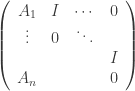
$\left(\begin{array}{cccc}A_1&I&\cdots & 0\\ \vdots & 0& \ddots & \\ & & &I\\ A_n & &&0\end{array}\right)$
where each entry represents a 2×2 block and $A_1$ is trace free. This is a transverse slice to the (n,n) nilpotent matrices. Let $\chi: M\to \mathbb{C}^{2n-1}$ take each matrix to the coefficients of its characteristic polynomial. The define $Y_n$ to be the preimage of a generic point of $\chi$ . We can map $\mathbb{C}^{2n-1}$ to $Sym^{2n}_0(\mathbb{C})$ , the space of unordered 2m tuples of complex numbers whose sum is 0, by sending the corresponding characteristic polynomial of the traceless matrix to its eigenvalues. For each point $\tau \in Conf^{2n}_0(\mathbb{C}) \subset Sym^{2n}_0(\mathbb{C})$ where all of the eigenvalues are distinct, there is a corresponding fiber $\chi^{-1}(\tau)=Y_n^{\tau}$ . Parallel transport around loops in $Conf^{2n}_0(\mathbb{C})$ defines a representation from the braid group to $\pi_0(Symplectomorphisms(Y_n^{\tau_0}))$ .

Next, look at the Lagrangian intersection Floer homology in this space $Y_n^{\tau_0}$ . It is a theorem of Seidel and Smith that there exists a Lagrangian submanifold $L\cong(S^2)^n\subset Y_n^{\tau_0}$ such that $HF^*(L,(\beta \times id)(L))$ is an integer graded link invariant for a braid, $\beta\in Br_n$ . They expect this to agree with Khovanov homology, where the integer grading coming from the Floer homology agrees with the difference between the Alexander and Maslov gradings in Khovanov homology.

Here is a way to understand the Lagrangian L. Manolescu constructed an open embedding from $Y_n$ into $Hilb^n(X_n)$ , where $X_n$ is the Milnor fiber $X_n=\{x^2+y^2+z^{2n}=1\}\subset \mathbb{C}^3$ , and $Hilb^n(X_n)$ is a resolution of $Sym^n(X_n)$ at the singularities along the diagonal. Since $X^n\subset \mathbb{C}^3$ , there is a projection $\pi_z: X_n\to \mathbb{C}$ projecting onto the last complex coordinate. This projection has some critical values at the roots of $z^{2n}-1$ , above which the fibers are singular cones. Above the regular values, the fibers are cylinders. If one draws a path between two critical values in $\mathbb{C}$ , and looks at the vanishing cycles in the corresponding fibers you see a sphere as in the picture below.

Lefschetz Fibration

To get $(S^2)^n$ , you take n disjoint paths in $\mathbb{C}$ between critical values, i.e. a crossingless matching of 2n points. Taking the preferred crossingless matching which matches the ith point to the (2n-(i-1))th point for $1\leq i \leq n$ , gives the Lagrangian L of the theorem. Note that this was also the preferred crossingless matching in Khovanov’s algebraic construction.

One can form the analog of the arc algebra in this symplectic setting in the following way. For crossingless matchings A and B, let $L_A$ and $L_B$ be the associated Lagrangians. Then define $H_n^{symp}=\sum_{A,B}HF^*(L_A,L_B)$ where the Floer Homology is taken in $Y_n$ . There is an expectation that $H_n^{symp}=H_n$ , and this was proven over $\mathbb{Z}/2$ by Rezazadegan.

Next one would like to analyze what happens when you look at $\chi^{-1}(\tau_{sing})$ when $\tau_{sing}$ is no longer a regular value of the characteristic polynomial map. Start out with the simplest kind of singularities when only two eigenvalues coincide. Seidel and Smith show that the singular locus of this fiber can be canonically identified with $Y_{n-1}$ as two eigenvalues come together to one in $Y_n$ . Transverse to the singular locus is n=1 Milnor fiber, which has a vanishing cycle giving rise to an $S^2$ . Thus colliding $(i,i+1)$ critical points give rise to a Lagrangian $\Gamma_i\subset Y_{n-1}\times Y_n$ , where $Y_{n-1}$ . (There are some holes in what I’ve said here, but I’m not sure yet how to fill them in.)

In the end, they obtain a Fukaya category from $Y_n$ , $\mathcal{F}(Y_n)$ , and bimodules defined by the Lagrangians $\Gamma_i$ between $\mathcal{F}(Y_{n-1})$ and $\mathcal{F}(Y_n)$ . They build up a symplectic cube of resolutions using long exact sequences in Floer theory for fibered Dehn twists, where the edges and diagonals are defined by the differential and higher products in the Fukaya category. To show that this is isomorphic to the original Khovanov homology, they want to show that these Fukaya categories are “formal” meaning equivalent to a minimal $A_{\infty}$ algebra whose higher products vanish. Abouzaid explains this in more detail in part two of this talk, below.

Symplectic Khovanov Part 2

Chapter 3: Recovering the bigrading

Lagrangian Floer homology has a single grading, but Khovanov homology is bigraded. It requires some effort to recover the second grading on the symplectic Khovanov homology side. The first step is to partially compactify the space $Y_n$ by adding in some divisor D. In the Milnor fiber $X_n$ , you should add in two points at infinity to each fiber in the Lefschetz fibration so that the cylindrical fibers become spheres and the cone fibers become a wedge of two spheres. Use this and the embedding of $Y_n$ into $Hilb^n(X_n)$ to define the appropriate partial compactification of $Y_n$ . Now we have a manifold $\overline{Y} = Y_n\cup D$ . Choose a perturbation $D_{\varepsilon}$ of D in $\overline{Y}$ .

They define $\Delta^0 \in HF^1(L,L)$ by counting points on disks with boundary along L, which intersect $D$ and $D_{\varepsilon}$ each in a unique point, as in this picture.

$disks defining $\Delta_0$ and $\Delta_1$$

Disks defining $\Delta_0$ and $\Delta_1$.

This is well defined when some Gromov-Witten invariant of $\overline{Y}$ vanishes. In the case that $\Delta^0$ vanishes, they call L infinitesimally invariant. If $(L_0,L_1)$ are infinitesimally invariant Lagrangians, it is possible to define a relative bigrading on $HF^*(L_0,L_1)$ . The first grading is just the homological grading, and the second grading is a weight determined by a certain map $\Delta^1: HF^*(L_0,L^1)\to HF^*(L_0,L_1)$ . For $x\in HF^*(L_0,L_1)$, which can be represented by an intersection point between the two Lagrangians, we define $\Delta^1(x)$ by the picture above, by counting all disks with boundary along $L_0$ and $L_1$ containing x in the boundary and a summand of $\Delta^1(x)$ at the other intersection of the Lagrangians on the boundary, with the condition that the interior of the disk intersects D and $D_{\varepsilon}$ each in a unique point (see picture). To obtain the relative grading, decompose $HF^*(L_0,L_1)$ by the generalized eigenvalues of $\Delta^1$ . Some bubbling issues prevent this from being an absolute grading without some additional choices, but this can be fixed by making some cohomology choices. Although the resulting absolute grading is not a priori integral, it is integral in practice.

There are similarly defined $\Delta^i$ for each $i\in \mathbb{N}$ , and these are needed to show that the weight grading is compatible with multiplication.

Chapter 4: Formality

An $A_{\infty}$ algebra is a differential algebra whose multiplication is not quite associative, but is endowed with higher product operations which describe the homotopies that describe the failure of associativity of the lower products. The product operations are called $m_1,m_2,m_3,\cdots$ , where $m_1$ is the differential, $m_2$ is a product, $m_3$ is the homotopy showing $m_2$ is associative on the level of homology, etc. An $A_{\infty}$ algebra is called minimal if $m_1\equiv 0$ . It is a theorem that every $A_{\infty}$ algebra is equivalent to a minimal one. An $A_{\infty}$ algebra is called formal if it is equivalent to a minimal algebra whose higher products, $m_3,m_4,\cdots$ all identically vanish. They show that the symplectic arc algebra C is formal by using the class $\Delta=\{\Delta_i\}\in HH^1(C,C)$ . I am lacking some of the algebraic knowledge to say much more about what these objects are or how the proof of this part goes.

Once formality is established, the symplectic cube would correspond to Khovanov’s cube of resolutions, so the spectral sequence from Khovanov homology to Symplectic Khovanov homology would degenerate immediately, and the two theories would be isomorphic. This would provide and interesting link between symplectic geometry and Khovanov’s more combinatorial formulation of the link invariant. I would be interested to see what kinds of new information we can obtain about Khovanov homology from the symplectic version, or what we can learn about symplectic geometry from Khovanov homology.

1 Comment

Filed under Conference Notes

by Peter Lambert-Cole | July 20, 2012 · 3:03 pm

Budapest Research Talks: Tuesday

Frederic Bourgeois: The Geography of Legendrian submanifolds
Frederic’s talk focused on Legendrian submanifolds in 1-jet spaces that arise from generating families of functions. A simple way to create Legendrian submanifolds in $J^1(M) = T^*M \times \mathbb{R}$ is to look at the graph in $J^1(M)$ of a smooth function f on M. However, this is a trivial example because all such Legendrians are isotopic to each other through Legendrians, including Legendrian isotopic to the 0-section. A subtler construction is through generating families. Here, we take a smooth function F on $M \times \mathbb{R}^n$ , which we can think of as a family of smooth functions on M parametrized by $\mathbb{R}^n$ . If we let $\Sigma$ be the critical set of the F, then we can map $\Sigma$ into $J^1(M)$ as a Legendrian by $(x,e)\mapsto (x,\frac{\partial F}{\partial x}(x,e), F(x,e))$ .

There are two operations for generating families F for a Legendrian L that define an equivalence relation. We can stabilize, meaning we extend F to a function on $M \times \mathbb{R}^{n+1}$ in a trivial manner, and we can precompose F with a fiber diffeomorphism that maps each vector space $\mathbb{R}^n$ to itself.

We can also define an invariant of the pair (L,F), called generating family homology, as follows. Take the difference function $\Delta(x,e,e') = F(x,e) - F(x,e')$ , defined on $M \times \mathbb{R}^{2n}$ . There is a one-to-one correspondence between critical points at positive critical values and Reeb chords of L. If we let $\Delta^a = \{(x,e,e')| \Delta(x,e,e') < a \}$ and choose some $\delta >0$ small than the length of any Reeb chord, we can define our invariant to be the relative homology $GFH(L,F) = H_*(\Delta^{\infty},\Delta^{\delta})$ , which really is invariant up to the equivalence relation mentioned above.

This is starting to look like Legendrian Contact Homology, as GFH is a homology invariant whose generators are Reeb chords. In fact, for Legendrian knots, GFH is equivalent to the linearized LCH of L for some augmentation of the dg-algebra. An augmentation $\epsilon$ is a ring homomorphism from an algebra A to a field that nicely splits the differential into a graded morphism. We obtain a new map $\partial^{\epsilon}$ that sends each word of k letters $b_1b_2 \dots b_k$ to some linear combination of words, each still with exactly k letters. Let $m(a,b_1,\dots,b_2)$ be the sum over $\mathbb{Z}/2$ of punctured curves mapping the boundary of the disk to L and the punctures to $a, b_1,\dots,b_n$ , as is standard in LCH. Then the new map is $\partial^{\epsilon}(a) = \sum_{b_{i_1},\dots , b_{i_k}} \sum_{j=1}^k m(a,b_{i_1},\dots , b_{i_k}) \epsilon(b_{i_1}) \dots \epsilon(b_{i_{j-1}}) b_{i_j} \epsilon(b_{i_{j+1}}) \dots \epsilon(b_{i_k})$ .

Moreover, it restricts to a differential on the 1-graded piece, the single letter words that correspond 1-1 with our Reeb chords. The homology of this is much simpler than the homology of the whole dg-algebra and we can encode the ranks of our the homology groups of this chain complex in a Poincare polynomial. Now, not every Legendrian knot admits an augmentation on is DGA, but if L is constructed from a generating family, then there exists a unique choice of augmentation and every augmentation comes from some generating family. Fuchs and Rutherford have proved that GFH is in fact graded isomorphic to linearized DGA.

A more powerful invariant can be obtained by considering two augmentations at once, using the following linearization:

$\partial^{\epsilon_1, \epsilon_2}(a) = \sum_{b_{i_1},\dots, b_{i_k}} \sum_{j=1}^k m(a,b_{i_1},\dots, b_{i_k}) \epsilon_1(b_{i_1}) \dots \epsilon_1(b_{i_{j-1}}) b_{i_j} \epsilon_2(b_{i_{j+1}}) \dots \epsilon_2(b_{i_k})$ .

This is more powerful because it keeps track of the order that Reeb chords appear at punctures for a disk. Similarly, we could consider a difference function $\Delta' = F_1(x,e) = F_2(x,e')$ for two different generating families $F_1,F_2$ and obtain a homology $GFH(L,F_1,F_2)$ . They prove that these two homologies are in fact equivalent.

As a final question, he discussed what Poincare polynomials of linearized LCH can occur. He cited a result due to Ekholm, Etnyre and Sabloff that established a form of Poincare duality for LCH and defined a double compatible Laurent polynomial as any polynomial that could be the Poincare polynomial of a complex whose homology satisfies the above condition. He, Sabloff and Traynor have proved that for any given doubly compatible polynomial, there exists some Legendrian and an augmentation such that the Poincare polynomial of the linearized LCH is exactly the specified one.

Jacob Rasmussen:

Jacob’s talk investigated a conjecture that the Khovanov-Rozansky homology of a torus knot T(m,n) can be constructed using finite dimension representations of so-called rationals DAHAs (or double affine Hecke algebras; also referred to as Cherednik algebras). I’m not an expert on Khovanov homology and the actual statement of the conjecture seems too subtle for me to correctly reproduce. But I will try to state what seems to be the general idea.

The rational DAHAs are deformations of the familiar Weyl algebra. The Weyl algebra is the ring of differential operators on the polynomial ring $R = \mathbb{C}[x_1,\dots,x_n]$ with polynomial coefficients. It is generated by the operators $x_i$ , corresponding to multiplication by $x_i$ , and $\partial/\partial x_i$ , corresponding to partial differentiation with respect to $x_i$ . These operators commute except for $[\partial/\partial x_i, x_i] = id$ ; this is just an elementary calculation in calculus and is a manifestation of the so-called canonical commutation relation. This algebra is simple, meaning it has no nontrivial left or right ideals, and so it has no finite-dimensional representations.

However, we can deform the Weyl algebra by replacing the partial differential operators with Dunkl operators

$D_i f = \frac{\partial f}{\partial x_i} + c \sum_{j \neq i} \frac{s_{i,j} (f)-f}{x_i-x_j}$ .

where c is some complex number and $s_{i,j}$ is the involution on $\mathbb{C}[x_1,\dots,x_n]$ that switches the two indeterminates $x_i \leftrightarrow x_j$ . Clearly, setting c equal to 0 gives us the original Weyl algebra.

Interestingly, these deformed algebras do admit finite dimensional representations if $c = m/n$ for some integer coprime to n. The vector space $L_{m/n}$ on which it acts can be realized as a quotient of R by a homogeneous ideal of polynomials of degree less than or equal to m.

If we let V denote the linear polynomials in R, then the conjecture states that

$\bar{H}(T(m,n)) \cong (\Lambda*V \otimes_{Gr} L_{m/n})^{S_n}$

i.e. the $S_n$ -invariant elements of the associated graded of the exterior algebra of V tensored with the representation $L_{m/n}$ . The a-grading should be sent to the grading in the exterior algebra, the q-grading should be sent to the degrees of polynomials in $L_{m/n}$ and the t-grading should be sent to the associated graded of a filtration on $L_{m/n}$ .

Leave a comment

Filed under Conference Notes

by lstarkston | July 20, 2012 · 11:05 am

Naturality in Heegaard Floer homology

Andras Juhasz gave a talk yesterday afternoon on the naturality of HF. Naturality is a subtle issue that can be easily overlooked. The upcoming related paper is joint with Ozsvath and D. Thurston. The issue is that Heegaard Floer homology associates abelian groups to a 3-manifold which are only well defined up to isomorphism. If you want to be able to compare specific group elements of $HF^{\circ}(Y)$ where the elements are defined by distinct Heegaard diagrams $H_1,H_2$ , you need a canonical isomorphism from $HF^{\circ}(H_1)$ to $HF^{\circ}(H_2)$ that tells you whether the element defined using Heegaard diagram $H_1$ corresponds to the same element defined using Heegaard diagram $H_2$ . Their project is to construct these isomorphims, and decide how much data must be fixed in order for these maps to be canonical. Fortunately for those using Heegaard Floer homology, there are such canonical isomorphisms when you fix some small amount of data. A particularly useful application of these canonical isomorphisms is that it would allow direct comparison of the contact invariant for different contact structures on a given 3-manifold. This would give stronger results when both contact structures had nonvanishing contact invariant, and no easily distinguishable algebraic properties.

The theorem is as follows. Let $Man_*$ be the category of based 3-manifolds with basepoint preserving diffeomorphisms. Then there is a functor from $Man_*$ to the category of $\mathbb{F}_2$ vector spaces, which is isomorphic to $\widehat{HF}$ as originally defined by Ozsvath and Szabo. In other words, if H and H’ are two Heegaard diagrams for a 3-manifold Y, and d is a diffeomorphism of Y taking H to H’ fixing the basepoint, then there is a canonical isomorphism induced on the Heegaard Floer homology. Loops in the space of Heegaard diagrams with fixed basepoint induce the identity isomorphism. There is also a version for link Heegaard Floer homology.

Note that these Heegaard diagrams are considered as embedded into the 3-manifold Y, not just abstract Heegaard diagrams. For two Heegaard diagrams which are abstractly the same, but embedded in different ways, we must find a diffeomorphism of Y taking one embedding to the other, and there will be an induced isomorphism on the Heegaard Floer homology.

One important issue Juhasz mentioned, is that in the Heegaard diagram $(\Sigma, \alpha, \beta, z)$ , $\Sigma$ should be considered an oriented surface, since there are examples of diffeomorphisms taking a Heegaard diagram to itself, but reversing orientation on $\Sigma$ that induce a nontrivial isomorphism on the Heegaard Floer homology. The example Juhasz gave is for $S^2\times S^1$ with a torus Heegaard diagram. See the picture below.

Heegaard diagram for S^2xS^2

A $180^{\circ}$ rotation about the axis shown reverses the orientation of the torus, and switches the two generators of the Heegaard Floer homology, thus giving a nontrivial isomorphism induced by a loop in the space of Heegaard diagrams.

An additional requirement is that the diffeomorphism must fix the basepoint, at least for the hat version of Heegaard Floer. A simple example showing the necessity of this condition is a lens space L(p,1) with a standard Heegaard diagram on a torus (identified with $\mathbb{R}^2/\mathbb{Z}^2$ ) with a horizontal alpha curve and a beta curve of slope p. A horizontal translation by 1/p induces a permutation of the p intersection points which generate $\widehat{HF}$ , however such translations do not fix the basepoint.

Given these requirements, they are able to show naturality of Heegaard Floer homology. Here is some idea of the proof. Given two Heegaard diagrams H and H’ and some diffeomorphism $d: H\to H'$ we want to construct a unique map $\phi_{H,H'}: HF(H) \to HF(H')$ . For any two Heegaard diagrams H and H’, we can find a sequence $H\to H_1 \to \cdots \to H_n=H'$ where each arrow is one of the following:

an isotopy of $\alpha$ or $\beta$ curves
a handleslide
a stabilization/destabiliation
an isotopy of $\Sigma$ in Y

They construct an isomorphism on the Heegaard Floer homology for each of these moves and then define $\phi_{H,H'}$ as the composition of all these isomorphisms. To show naturality, they need to show that $\phi_{H,H'}$ does not depend on intermediate choices. This means that any loop from a Heegaard diagram back to itself, should induce the identity map. To show this I think the idea is to find a set of generators of nontrivial loops through Heegaard diagrams, and prove that for each of these generators the map induced on Heegaard Floer homology is the identity. One example of a generator given at the end of the talk is shown in the picture in this link.

A sequence of Heegaard diagram moves in a loop.

The first arrow going down and the second arrow pointing up to the right are handleslides, and the last arrow going up to the left is an isotopy back to the original Heegaard diagram. The idea is then to compute the isomorphisms corresponding to the handleslides and isotopies and prove that they compose to give back the identity.

Juhasz mentioned there are 14 cases to check like the above double handleslide-isotopy loop. Then it seems like you should use commutativity relations of the above four moves to determine that all loops can be reduced to products of these 14 loops.

Leave a comment

Filed under Conference Notes

by lstarkston | July 16, 2012 · 3:58 pm

Budapest Research talks: Monday

Tobias Ekholm gave a talk today entitled Exact Lagrangian immersions with a single double point. The relevant paper on the arXiv has the same name and is joint between Ekholm and Ivan Smith. The following is based on my notes from the talk and discussions that followed. The motivating question here is how much information we can obtain about the smooth structure of a manifold by looking at the symplectic topology of its cotangent space.

First, the definition of an exact Lagrangian immersion… A Lagrangian immersion $f:K\to (X,\omega)$ is an immersion such that $f^*\omega=0$ . An exact symplectic manifold has $\omega=d\lambda$ . Note that the standard symplectic structures on $T^*M$ and $\mathbb{C}^n$ are exact. Finally, an exact Lagrangian immersion is a Lagrangian immersion into an exact symplectic manifold such that $f^*\lambda =0$ .

Because the zero section $T^*M$ (with the standard symplectic structure) is an exact embedded Lagrangian, studying the smooth topology of M via the symplectic topology of $T^*M$ exact Lagrangian embeddings into standard symplectic manifolds. One simple property of a manifold that can be detected in this way is whether the manifold is closed (in the topologist sense i.e. compact without boundary). Gromov proved that there are no exact Lagrangian embeddings of a closed manifold into $\mathbb{C}^n=T^*\mathbb{R}^n$ . You can see this easily in the n=1 case: if you had an embedded exact closed Lagrangian curve in the plane: $\gamma: S^1\to \mathbb{C}$ , it encloses some region D. By Stokes’ theorem

$\int_D dx\wedge dy = \int_{\gamma}-ydx = \int_{S^1}\gamma^*(-ydx) =0$
therefore any closed exact Lagrangian in $\mathbb{C}$ (or more generally $\mathbb{C}^n$ ) must have self-intersection points. Ekholm and Smith try to push this further, to eliminate the possibility of exact Lagrangian immersions into $\mathbb{C}^n$ with a single double point. There is a necessary restriction on Euler characteristic, but otherwise they show that the sphere with its standard smooth structure is the only manifold with such an immersion. Formally, the theorem is:

Theorem: If K is a closed oriented 2k-manifold for $k>2$ with $\chi(K)\neq -2$ , which admits an exact Lagrangian immersion $f: K\to \mathbb{C}^{2k}$ then K is diffeomorphic to $S^{2k}$ the standard 2k-sphere.

This means that we get information about exotic even dimensional spheres by studying the symplectic topology on $\mathbb{C}^n$ .

Note, the Euler characteristic restriction is necessary (there are counterexamples).

Here are some of the main ideas that come up in the proof of the theorem.

Step 1: Use some older results coming from symplectic field theory, to say that K is necessarily a homotopy sphere. Somehow the exact Lagrangian immersion f gives rise to a dga generated by the unique double point. The Euler characteristic restriction is necessary at this point to switch to linearized contact homology. This is used to show K is a homology sphere, and doing a harder version of all this shows that K is actually a homotopy sphere.

Step 2: Resolve the double point by Lagrangian surgery to a new exact Lagrangian embedding of a manifold L. The resolution is locally modeled on the following setup. The double point is the origin at the intersection of $\mathbb{R}^n$ with $i\mathbb{R}^n$ in $\mathbb{C}^n$ . Remove a disk around the origin and smooth in one of two possible ways, so that the resulting manifold is K with a 1-handle attached. Of course you have to show that you can do this in a Lagrangian way (construction due to Polterovich).

Step 3: Form a moduli space of curves $u: D\to \mathbb{C}^n$ such that $u(\partial D)\subset L$ and u satisfies a perturbed version of the Cauchy-Riemann equations. These equations include a parameter j. When j=0, the solutions to the perturbed equations are just the constant solutions of maps into L. As j is sent to infinity, eventually the moduli space of solutions becomes empty. The idea is that the set of all solutions forms a symplectic filling of the exact Lagrangian L. Unfortunately, there are some singularities to deal with. Resolving these singularities is pretty subtle, but Ekholm and Smith manage to get some restrictions on how bad things can get, in particular they can only have bubbling phenomena with 2 bubble components. Eventually they are able to change this moduli space into a smooth stably parallelizable filling of L (stably parallelizable means that if you direct sum the tangent bundle with a trivial bundle, you get a trivial bundle).

Step 4: After adding a cancelling 2-handle to get back to a manifold with boundary our unsurgered manifold K, we obtain a stably parallelizable filling of K. By results that date back to 1967 by Kervaire and Milnor, this stably parallelizable filling suffices to show that K has standard diffeomorphism type.

Further thoughts…

This theorem is stated only for even spheres of dimension strictly greater than 4. It seems likely that the proof fails on many levels if you try to apply it to 4-manifolds, but it seems like an interesting question to ask whether any of these ideas can be applied to studying the smooth Poincare conjecture in dimension 4, or understanding other exotic 4-manifolds based on their embeddings/immersions into symplectic manifolds.

Leave a comment

Filed under Conference Notes

by Peter Lambert-Cole | July 15, 2012 · 11:44 am

Live from Budapest

From July 9-20, we’re at the CAST (Contact and Symplectic Topology) 2012 summer school and conference at the Alfred Renyi Institute of Mathematics in Budapest, Hungary. The format is two mini-courses per week along with two research talks every afternoon.

First Week:

Robert Lipshitz – Bordered Heegaard Floer Homology (lecture notes)

This week, Robert lectured on a Heegaard Floer-like structure associated to bordered 3-manifolds, which was constructed by himself, Peter Ozsvath and Dylan Thurston. This associates two modules, $\hat{CFA}(Y), \hat{CFD}(Y)$ to a 3-manifold with connected boundary, depending upon whether we think of the boundary as positively or negatively oriented. There are also more complicated modules associated to the nonconnected boundary case that mixes -A and -D structure. The main theorem is the Pairing Theorem (LOT), which states that for $Y = Y_1 \cup Y_2$ then $\hat{CF}(Y) = \hat{CFA}(Y_1) \otimes \hat{CFD}(Y_2)$ where $\hat{CF}$ is the chain complex for the hat version of Heegaard Floer. For the first three days, he developed the terminology and combinatorics of parametrizations of the boundary $\partial Y$ , defined the differential and discussed the relevant moduli of holomorphic curves. One key aspect of this construction is that it relies on his cylindrical reformulation of HF to bring it more in line analytically with Symplectic Field Theory. The fourth day, Jen Hom went over how to compute $\hat{CFA}(Y)$ for knot complements and the fifth day Robert discussed computing $\hat{CFA}(Y)$ for mapping tori and that it may be possible to simplify computations of $\hat{HF}(Y)$ by computing the bordered version for generators of the mapping class group and composition of these elementary cobordisms.

Kai Cieliebak – Stein Structures: Existence and Flexibility (lecture notes)

The subject of this talk was building Stein structures and classifying them up to the appropriate homotopy equivalence. Most of the content comes from an upcoming textbook on Stein structures written by Cieliebak and Yasha Eliashberg. A Stein manifold is a complex manifold that embeds properly, holomorphically into some $\mathbb{C}^n$ ; equivalently, it admits an exhausting (proper, bounded below), J-convex (or strictly plurisubharmonic) function $\phi$ , which can be used to set up the embedding into affine space. An important result, which is due to Milnor and can be verified easily, is that the Morse index of a nondegenerate critical point of $\phi$ must be less than or equal to $n$ . The goal of the lecture series is to prove the converse, that if an open, smooth, oriented manifold $M$ of dimension $2n > 4$ admits an almost complex structure $J$ and a generic Morse function $\phi$ with critical points of index less than $n$ , then there is a homotopy of almost-complex structures from $J$ to some $J'$ so that $\phi$ is $J'$ -convex, giving a Stein structure. The basic idea is to use a Stein h-cobordism theorem to simplify the set of critical points and attaching spheres of handles, build a model J-convex structure on a handles and extend the standard Stein structure on the unit ball as we add on handles. The last issue is flexibility and classifying Stein structures up to Stein homotopy. In the subcritical case, it follows from the h-principle for isotropic embeddings that if two Stein structures $(V,J), (V',J')$ have homotopic almost-complex structures then they are Stein homotopic. This is enough for the subcritical case, when $M$ has the homotopy type of an $n-1$ -dimensional manifold. The critical case relies on Max Murphy’s notion of loose legendrians, which do satisfy an h-principle. A Stein structure is flexible if its critical attaching spheres are loose, and flexible Stein structures with homotopic almost-complex structures are in fact Stein homotopic.