This is my summary of Yasha Eliashberg’s minicourse. The topic is contact and symplectic homology invariants of Weinstein manifolds, and the effects of handle attachments. I think the theories are too complicated to explain all the details in 3 talks, so if you really want to compute these things, look at the paper by Bourgeois, Ekholm, and Eliashberg here: http://arxiv.org/pdf/0911.0026v4.pdf
Part I: Weinstein manifolds
The goal is to compute invariants of Weinstein manifolds. A Weinstein manifold consists of the following data:  where
where
–  is an exact symplectic manifold with primitive
  (
( )
)
– Z is a complete vector field such that  (note Z and
  determine the primitive )
–  is an exhausting function (proper and bounded below)
– Z is gradient-like for 
Note that  and is equivalent to
  . We say in this case that Z is a Liouville vector field. Also note, X is necessarily noncompact since it is an exact symplectic manifold (Stokes theorem).
We will restrict to Weinstein manifolds of finite type, meaning has finitely many critical points. This means that there is some regular value c, such that all critical values are less than c. In this case, has a conical end,  . Therefore it is frequently interesting to just look at
 ![\overline{X}=\phi^{-1}((-\infty, c])](https://s0.wp.com/latex.php?latex=%5Coverline%7BX%7D%3D%5Cphi%5E%7B-1%7D%28%28-%5Cinfty%2C+c%5D%29&bg=ffffff&fg=333333&s=0&c=20201002) , such things are called Weinstein domains. One can also consider Weinstein cobordisms:
, such things are called Weinstein domains. One can also consider Weinstein cobordisms: ![\phi^{-1}([c_1,c_2])](https://s0.wp.com/latex.php?latex=%5Cphi%5E%7B-1%7D%28%5Bc_1%2Cc_2%5D%29&bg=ffffff&fg=333333&s=0&c=20201002) for regular values
for regular values  .
.
For any regular level set of the Weinstein structure function  , the restriction of is a contact form:
  must be positive on a basis for
  since the span of Z is the kernel of
  , and Z is transverse to the regular level sets.
There is some question of whether you can generally perturb the Weinstein structure to ensure is a Morse function, but in the case where it is Morse, you can consider the stable manifold of a critical point. Such stable manifolds are isotropic for both and (i.e. the restriction of the primitive to the stable manifold is zero). This implies that the indices of all critical points of are at most half the dimension of X. The intersection of the level sets with the stable manifolds are isotropic in the contact sense.
A question we would like to understand is how does the Weinstein manifold change as we pass through critical points of . Topologically we are doing a handle attachment, and the geometric information we get is that the attaching sphere will be isotropic in the contact sense, and the core of the handle will be isotropic in the symplectic sense. The framing on a Legendrian attaching sphere (for middle dimensional handles) is completely determined when the contact structure is co-oriented.
We can understand Weinstein manifolds and their invariants piece by piece for each handle addition. To use this method it is useful to establish a lemma that allows one to reorder the critical points, without meaningfully changing the Weinstein structure. One main reason for this is that all of the interesting symplectic geometry happens when attaching the n handles in a 2n dimensional manifold, so we want to attach all the k<n handles first and then focus on what happens when attaching the n-handles. Here, noninteresting means that h-cobordism principles hold, so information about the tangent bundle determines the symplectic manifold. There are also certain Legendrian attaching spheres (called loose) for n-handles for which the Weinstein manifold is determined homotopically (information about the tangent bundle determines the symplectic manifold).
Part II: Invariants of Weinstein manifolds: Symplectic and Contact homology
Set up: Let be a Weinstein manifold of finite type, ![\overline{X}=\phi^{-1}((-\infty,c])](https://s0.wp.com/latex.php?latex=%5Coverline%7BX%7D%3D%5Cphi%5E%7B-1%7D%28%28-%5Cinfty%2Cc%5D%29&bg=ffffff&fg=333333&s=0&c=20201002) be a Weinstein domain such that X is
be a Weinstein domain such that X is  union a conical end, and let
  . We will build up some chain complexes that are invariants of the Weinstein manifold X.
Reeb orbits: the first basic generators of the chain complex will be Reeb chords and periodic orbits of the Reeb vector field associated to on Y. It is convenient for the following to assume  . For each periodic Reeb orbit there is a Conley-Zehnder index, there is also a well-defined index associated to Reeb chords. There is some distinction between “good” Reeb orbits and “bad” ones. A bad Reeb orbit is an even multiple of another Reeb orbit, such that the parity of the Conley-Zehnder index can change as one takes different multiples of the simple Reeb orbit. Orbits that are not bad are good. These bad orbits introduce some additional problems one needs to compensate for to get a well defined theory.
Linearized contact homology  : While this invariant is meant to give information about the contact manifold Y, it depends on the choice of a Weinstein filling X. The chain complex for linearized contact homology is generated (over some field of characteristic 0) by the set of all good Reeb orbits.
The differential for contact homology: The coefficient  is a count of holomorphic “cylinders” in the symplectization of Y connecting
  to
to  . The quotations are because we must count curves that have additional ends on the negative end besides just , when these additional ends can be capped of by holomorphic disks in the filling , of Y. These curves are called cylinders anchored in the symplectic filling.

Note that this is where the dependence on X for contact homology comes from. Counting these anchored cylinders is necessary to get the differential to square to zero since these appear as ends of the moduli space.
Reduced Symplectic Homology,  : While contact homology ignores the bad vertices, we can obtain additional information by including the bad vertices and compensating for their bad behavior in the differential. To do this we take two direct sum copies of the module generated by all Reeb orbits. We indicate orbits are in the first copy by putting a check over them, and in the second copy by putting a hat over them. Additionally, the elements in the second copy have grading shifted by 1.
  , where
 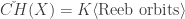 and
and ![\widehat{CH}(X) = K\langle \text{Reeb orbits}\rangle[1]](https://s0.wp.com/latex.php?latex=%5Cwidehat%7BCH%7D%28X%29+%3D+K%5Clangle+%5Ctext%7BReeb+orbits%7D%5Crangle%5B1%5D&bg=ffffff&fg=333333&s=0&c=20201002) .
.
The differential for plus symplectic homology: Since there are two direct summands in the chain complex  , we write the differential in block matrix form:
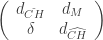 .
.
Here  are the differentials defined previously for CH by counting anchored cylinders.
 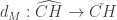 sends good hat orbits to zero, and for a bad orbit
  (this has something to do with the parity issues that bad orbits have). For each Reeb orbit, we will keep track of a marked point (so we have more data about the parametrization). The map
  counts holomorphic cylinders where the marks on the two Reeb orbits are aligned in the product, and also broken cylinders where the marked points show up in a chosen cyclic order as in the below picture.

Note that both of these are counts of a moduli space one codimension higher than the moduli space of unrestricted cylinders. I’m assuming all of these maps defined via counting curves are just summing over the 0-dimensional moduli spaces (or 1-dimensional moduli spaces mod an R-action).
Full Symplectic Homology,  : For this theory, we combine the symplectic homology chain complex which keeps track of Reeb orbits and holomorphic cylinders connecting them, with the Morse chain complex for
  , which keeps track of the handle attachments. The chain complex is given by
 ![SH(X) = SH^+(X) \oplus Morse(-\phi)[-n]](https://s0.wp.com/latex.php?latex=SH%28X%29+%3D+SH%5E%2B%28X%29+%5Coplus+Morse%28-%5Cphi%29%5B-n%5D&bg=ffffff&fg=333333&s=0&c=20201002) , where
, where  is the Morse chain complex generated by critical points of , whose differential counts gradient flowlines between critical points.
The differential for symplectic homology can again be defined by a block matrix in terms of the two summands:
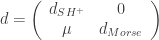
where here ![\mu: SH^+(X) =\check{CH}(X) \oplus \widehat{CH}(X) \to Morse(-\phi)[-n]](https://s0.wp.com/latex.php?latex=%5Cmu%3A+SH%5E%2B%28X%29+%3D%5Ccheck%7BCH%7D%28X%29+%5Coplus+%5Cwidehat%7BCH%7D%28X%29+%5Cto+Morse%28-%5Cphi%29%5B-n%5D&bg=ffffff&fg=333333&s=0&c=20201002) is defined by
is defined by  and
and  where
where  counts the number of holomorphic disks bounding
  whose center marked point maps into the stable manifold of p.
Note that since the differential for SH is lower-triangular, there is a short exact sequence of the complexes:  which induces an exact triangle on the level of homology:
  .
.
For , there is not quite an exact triangle between  since the differential is not triangular, so neither inclusions of
  or
or  into are chain maps. However since the map $d_M$ is zero on good orbits, we get an exact triangle
  when all Reeb orbits are good.
Part III: Computing Contact and Symplectic Homology
We want to compute these invariants via handlebody decompositions. Therefore we would like to know what the effect of attaching handle has on the Contact/Symplectic homology. The effects of adding subcritical handles (index <n) are basically trivial (the symplectic homology vanishes for Weinstein manifolds built from handles of index <n). Therefore we look at what happens to these homology invariants when attaching n-handles.
In the Weinstein manifold, the attaching spheres of the n-handles will be Legendrian submanifolds of the level set Y. There is an algebraic construction that captures the contribution of the n-handle to contact/symplectic homology in terms of the Legendrian attaching sphere. The construction is essentially a differential polynomial algebra  generated by the Reeb chords, with some extra formal variables added in. The differential is computed by correctly counting holomorphic disks with boundary along the Legendrian except at finitely many punctures which map to the Reeb chords. The details are probably more accurately described in the paper by Bourgeois, Ekholm, and Eliashberg, but the point is that there is a clear prescription on how to compute this once you understand the Reeb chords and some holomorphic disk counts of the Legendrian attaching sphere.
Now suppose  where h is an n-handle attached along a Legendrian
  . The theorem is that we get the complex for X, from the complex for
  and
and  ,
,  and the differential is given in block matrix form by
 .
.
Here the map  is zero on the hat part of SH. On the check part it counts holomorphic punctured disks, which send the puncture in the center asymptotically to the Reeb orbit
  , and maps the boundary of the disk to the Legendrian, except along finitely many points which map to Reeb chords showing up as a term in
  . (There is also a particular ray from to the boundary, which is kept track of through the formal structure of .) Finally on the Morse summand of the SH complex,
  counts some holomorphic disks that intersect the stable manifold of a critical point.
The payoff here is that there is an exact triangle relating  . In the case that has only handles of index <n, its symplectic homology vanishes, so we get an isomorphism
  . There are some additional techniques to obtain the computations of that involve looking at the corresponding algebra for the boundary of the cocore instead of the attaching sphere, and looking at some linearizations using augmentations handed to you by the Lagrangian filling of the Legendrian. Eliashberg thinks that such invariants are reasonable to compute, though that probably assumes one knows a lot about counting various kinds of holomorphic curves.

 . Yikes! The bordered techniques are computationally better, but require some rather difficult algebra.
 is a tree with integer weights
  associated to its vertices
  . We consider the plumbing construction
  . This means that
  is the compact oriented 4-manifold obtained by plumbing
  bundles over
  with Euler numbers given by the weights
  of the resulting manifold is our object of interest.
 to be
to be  mod 2 for all
  , i.e. the set of characteristic elements in the second integral cohomology group of
  denote the
 ![\mathbb{Z}_2[U]](https://s0.wp.com/latex.php?latex=%5Cmathbb%7BZ%7D_2%5BU%5D&bg=ffffff&fg=333333&s=0&c=20201002) module freely generated over
module freely generated over ![[K, E]](https://s0.wp.com/latex.php?latex=%5BK%2C+E%5D&bg=ffffff&fg=333333&s=0&c=20201002) , where
, where  is a characteristic covector and
  is a subset of vertices in
  .
.![\partial^-[K,E] = \Sigma_{v\in E} U^{a_v[K,E]} [K,E-v] + U^{b_v[K,E]} [K+2v^*,E-v]](https://s0.wp.com/latex.php?latex=%5Cpartial%5E-%5BK%2CE%5D+%3D+%5CSigma_%7Bv%5Cin+E%7D+U%5E%7Ba_v%5BK%2CE%5D%7D+%5BK%2CE-v%5D+%2B+U%5E%7Bb_v%5BK%2CE%5D%7D+%5BK%2B2v%5E%2A%2CE-v%5D+&bg=ffffff&fg=333333&s=0&c=20201002)
 and
and  are integers which are defined with an auxiliary function
  . If
. If  , then
 ![\mathcal{I}[K,I] = \frac{1}{2}(\sum_{u\in I}K(u) + (\sum_{u\in I}u)^2 )](https://s0.wp.com/latex.php?latex=%5Cmathcal%7BI%7D%5BK%2CI%5D+%3D+%5Cfrac%7B1%7D%7B2%7D%28%5Csum_%7Bu%5Cin+I%7DK%28u%29+%2B+%28%5Csum_%7Bu%5Cin+I%7Du%29%5E2+%29&bg=ffffff&fg=333333&s=0&c=20201002) . That second term represents a self-intersection in
. That second term represents a self-intersection in ![A_v[K,E] = \min\{ \mathcal{I} | I\subset E-v\}](https://s0.wp.com/latex.php?latex=A_v%5BK%2CE%5D+%3D+%5Cmin%5C%7B+%5Cmathcal%7BI%7D+%7C+I%5Csubset+E-v%5C%7D+&bg=ffffff&fg=333333&s=0&c=20201002)
![B_v[K,E] = \min\{ \mathcal{I} | v\in I\subset E\}](https://s0.wp.com/latex.php?latex=B_v%5BK%2CE%5D+%3D+%5Cmin%5C%7B+%5Cmathcal%7BI%7D+%7C+v%5Cin+I%5Csubset+E%5C%7D+&bg=ffffff&fg=333333&s=0&c=20201002)

 .
. , and compute all of the products
  . If:
. If: , then set
  and repeat.
 stands for both a vertex and the second homology class in the plumbed manifold corresponding to that vertex.) This algorithm produces a series of vectors
  , and terminates in finite time. The product, by the way, is a dot product computed in the intersection matrix of the four-manifold. I believe
  was a suggested example of a rational graph on which to perform the algorithm.
 such that sufficiently decreasing the weights
  makes
makes  rational.
 is a three-manifold invariant.
![\mathbb{HF}^-(G, \mathfrak{s}) \cong \mathbb{Z}_2[U]](https://s0.wp.com/latex.php?latex=%5Cmathbb%7BHF%7D%5E-%28G%2C+%5Cmathfrak%7Bs%7D%29+%5Ccong+%5Cmathbb%7BZ%7D_2%5BU%5D&bg=ffffff&fg=333333&s=0&c=20201002) for all spin-c structures over
for all spin-c structures over  .
. .
. converging to
  . If
. If  denote a plumbing graph with a distinguished, unweighted vertex
  . Define the lattice chain complex on
  . The vertex
 on the lattice homology complex. For a generator
 ![\mathcal{A}[K,E]](https://s0.wp.com/latex.php?latex=%5Cmathcal%7BA%7D%5BK%2CE%5D&bg=ffffff&fg=333333&s=0&c=20201002) is given by a formula that is essentially the same as the auxiliary function
is given by a formula that is essentially the same as the auxiliary function  is the subject of the main theorem:
 is negative definite* for
  . Then
  determines the lattice chain complex
 on the vertex
  is an L-space.)
 is a doubly filtered complex. The filtrations can be used to chop up the complex into various subcomplexes, and then these these subcomplexes, the maps relating them, and their mapping cones are used to describe the Heegard Floer of surgeries along
 ![\mathbb{CF}^\infty(G) = \mathbb{CF}^-(G)\otimes_{\mathbb{Z}_2} \mathbb{Z}_2[U^{-1}, U]](https://s0.wp.com/latex.php?latex=%5Cmathbb%7BCF%7D%5E%5Cinfty%28G%29+%3D+%5Cmathbb%7BCF%7D%5E-%28G%29%5Cotimes_%7B%5Cmathbb%7BZ%7D_2%7D+%5Cmathbb%7BZ%7D_2%5BU%5E%7B-1%7D%2C+U%5D&bg=ffffff&fg=333333&s=0&c=20201002) is doubly filtered by the action of
is doubly filtered by the action of  and an extension of
  are all rational, then the filtered chain complex of
  is equal to its knot Floer homology.
 ‘s. While knot concordance may not be able to tell us everything about smooth 4-manifolds, it can lead to interesting results. The goal then is to learn as much as possible about the size and structure of the concordance group.
![(S^1\times[0,1], S^1\times\{0,1\})\to (S^3\times[0,1], S^3\times\{0,1\})](https://s0.wp.com/latex.php?latex=%28S%5E1%5Ctimes%5B0%2C1%5D%2C+S%5E1%5Ctimes%5C%7B0%2C1%5C%7D%29%5Cto+%28S%5E3%5Ctimes%5B0%2C1%5D%2C+S%5E3%5Ctimes%5C%7B0%2C1%5C%7D%29&bg=ffffff&fg=333333&s=0&c=20201002) . This is an equivalence relation, and the space of knots modulo concordance equivalence forms an abelian group, (addition is connected sum, the unknot is the identity, and negation is the mirror image with reversed orientation). An equivalent definition for
. This is an equivalence relation, and the space of knots modulo concordance equivalence forms an abelian group, (addition is connected sum, the unknot is the identity, and negation is the mirror image with reversed orientation). An equivalent definition for  and
and  to be concordant is that
  is smoothly slice (bounds a disk in the 4-ball). We can also consider the topological concordance equivalence, which instead of requiring the above mapping of the cylinder to be smooth, we only require that it is continuous and extends to a continuous map on a tubular neighborhood. Topological concordance is a weaker equivalence than smooth concordance. Let
  denote the group of knots up to smooth concordance, and
  denote the group of knots up to topological concordance.
 . Showing that
  . Livingston, and Manolescu-Owens more recently showed that
  distinguished using the
  and
and  invariants from Heegaard Floer and Khovanov homologies, which are both concordance invariants.
 . The knots are Whitehead doubles of torus knots, and the proof uses SO(3) gauge theory to show the knots are not smoothly concordant.
 which can be computed from the chain complex
  through an algebraic process involving the
  induced by large integer surgeries on the knot in
  . The analog of addition in the knot concordance group is the tensor product of chain complexes by the following Kunneth formula:
  . If a knot K is smoothly slice, then
  . With the concordance equivalence relation, we started with a monoid of knots under connected sum, and mod out by the concordance equivalence relation to get a group. Similarly, the
  complexes form a monoid under tensor product and we obtain a group if we mod out by the equivalence relation
  . The resulting group
  has additional useful structure: a total ordering, a notion of much greater than, and a filtration. These structures can be used to show linear independence of knots in the concordance group.
 is defined, there is definitely a relation to the
  if and only if
  for every pattern P. Furthermore the satellite map descends to a well defined map on the group of knots up to
 ![\mathcal{C}_{\Delta} := \langle \{[K]: \Delta_K=1\}\rangle = \mathcal{C}_{TS}](https://s0.wp.com/latex.php?latex=%5Cmathcal%7BC%7D_%7B%5CDelta%7D+%3A%3D+%5Clangle+%5C%7B%5BK%5D%3A+%5CDelta_K%3D1%5C%7D%5Crangle+%3D+%5Cmathcal%7BC%7D_%7BTS%7D&bg=ffffff&fg=333333&s=0&c=20201002) ? The answer to this question is strongly no. Hedden and Livingston prove that there is an infinitely generated free abelian subgroup in the quotient:
? The answer to this question is strongly no. Hedden and Livingston prove that there is an infinitely generated free abelian subgroup in the quotient:  .
.![0=2[K]](https://s0.wp.com/latex.php?latex=0%3D2%5BK%5D&bg=ffffff&fg=333333&s=0&c=20201002) so
so ![[K]=-[K]=[\overline{K}^r]](https://s0.wp.com/latex.php?latex=%5BK%5D%3D-%5BK%5D%3D%5B%5Coverline%7BK%7D%5Er%5D&bg=ffffff&fg=333333&s=0&c=20201002) , i.e. the knot is isotopic to its reverse mirror image. Such knots have been studied for awhile, and are called amphichiral. There are lots of such knots, so it is reasonable to expect some of the topologically slice knots to have this property.
, i.e. the knot is isotopic to its reverse mirror image. Such knots have been studied for awhile, and are called amphichiral. There are lots of such knots, so it is reasonable to expect some of the topologically slice knots to have this property. .
. is keeping track of the highest grading of the generator of the nontorsion elements in the (minus) Heegaard Floer homology of a
  homology 3-sphere. To use this to obstruct sliceness, first one notices that if K were smoothly slice, then its branched double cover
  would be a
  (this comes from looking at the double branched cover of the 4-ball branched over the slice disk). This implies that the d-invariant
  for all spin-c structures on Y which are a restriction of a spin-c structure on Q. Since we are trying to obtain a contradiction, and show that such a Q does not exist, we don’t know exactly which spin-c structures will show up on the boundary. However such spin-c structures will satisfy certain properties (e.g. they form a subgroup of a certain size in
  . One can explicitly compute the d-invariants for the candidate 2-torsion knots, and look for possible spin-c subgroups satisfying the necessary conditions, and rule out the possibility that
  .
. . We can define an intermediate genus, called the concordance genus
  . One may ask what the possible size of the gaps can be in the inequality
  . The gap between concordance genus and slice genus can be made arbitrarily large by connect summing nontrivial slice knots, but it is more difficult to get gaps between
  and
and  . The first result regarding this problem is due to Nakanishi who found knots with concordance genus arbitrarily larger than 4-ball genus. Livingston improved this result and found algebraically slice (though not topologically slice knots) with
  but
but  for each
  .
. has a 1-dimensional submanifold of critical points, which map onto a 1-dimensional (almost) submanifold of Q, with finitely many cusps and crossings. This divides the base surface Q into “patches” (connected components of the complement of the critical values), divided by “seams” (the critical values except the cusps and crossings), plus some ends (discrete points at the crossings and cusps).
 to each patch
  , and a Lagrangian correspondence
  to each seam between patches
  . On the ends where multiple seams come together, one associates Floer homology classes. If you choose all of these things correctly, you can extract an invariant out of the 4-manifold. While it seems natural to me to build an invariant for a 4-manifold by gluing together simple pieces, it is not obvious where these symplectic manifolds and Lagrangian correspondences come from. It turns out the motivation is by looking at Donaldson theory in limiting cases.
 and look at the new anti-self dual equations with this metric as
  . It turns out that the solution space of connections in this limit is a symplectic space (there may be some singularities in general, but I think there are analytic assumptions one can make to avoid this). This is the motivation to associate a symplectic manifold to each patch.

 . See where those circles are sent under the diffeomorphism of
  . Check if the image of those circles bound disks in X’. If they do we can extend the diffeomorphism on the boundary over a neighborhood of these cocores. Then we are left with just extending a diffeomorphisms of
  over
over  . In the case that n=0, we are trying to extend a diffeomorphism of
  . The diffeomorphism probably extends, since if it doesn’t you get a counterexample to the smooth Poincare conjecture in dimension 4, so either way you should be happy.
 is a diffeomorphism. We glue the boundary of X to the boundary of Y handle by handle. First to glue the 0-handle of X to the 0-handle of Y requires an additional 1-handle connecting the two 0-handles. Since a standard diagram assumes a unique 0-handle in the background, we can cancel the new 1-handle with one of the 0-handles. To glue a 1-handle of X to a 1-handle of Y, we need to add a 2-handle that passes through each 1-handle. This would be straightforward if the diffeomorphism
  and
and  . Such diagrams apparently made it easy to read off the fundamental group of the manifolds, to confirm that they were simply connected and the constructions were actually the exotic manifolds they were suspected of being.
 which is an exotic copy of E(1). Akbulut constructs diagrams for E(1) where you can see the regular torus fibers explicitly and performs the log transforms then notices that much of the diagram for