This to-be-2-part-because-this-got-long post is a continuation of the series on Kylerec 2017 starting with the previous post, and covers most of the talks from Days 2-3 of Kylerec, focusing on the use of J-holomorphic curves in the study of fillings. I should mention that two more sets of notes, by Orsola Capovilla-Searle and Cédric de Groote, have been uploaded to the website on this page. So if you wish to follow along, feel free to follow the notes there, and in particular, the relevant talks I’ll be discussing in this post are:
Part 1
- Day 1 Talk 1 – The introductory talk by (mostly) Roger Casals (with some words by Laura Starkston)
- Day 2 Talk 2 – Roberta Gaudagni’s talk introducing J-holomorphic curves
- Day 2 Talk 3 – Emily Maw’s talk on McDuff’s rational ruled classification
Part 2
It should be obvious in what follows which parts of the exposition correspond to which talks, although what follows is perhaps a pretty biased account, with some parts amplified or added, and others skimmed or skipped.
J-holomorphic curves – basics
Gromov introduced the study of J-holomorphic curves into symplectic geometry in his famous 1985 paper, immediately revolutionizing the field. One might wonder why we care about these objects, and the rest of this post (along with part 2) should be a testament to some (but certainly not all) aspects of the power of the theory.
The “J” in “J-holomorphic” refers to some choice  of almost complex structure on a manifold
  . Given an almost complex manifold, a J-holomorphic curve is a map
  such that
  is a Riemann surface and
  . In the case where
  is a complex manifold, we see this is precisely what it means to be holomorphic.
We are mostly concerned a choice of which is compatible with a symplectic manifold  . By this, we mean that the (0,2)-tensor
  is a Riemannian metric. We say is tame if
  for each nonzero vector
  (note that
  as defined above is not necessarily symmetric in this case).
Proposition: The space of compatible almost complex structures on a symplectic manifold is non-empty and contractible. So is the space of tame almost complex structures.
This suggests either:
- Studying the space of J-holomorphic curves into
 for some particular choice of .
- Study some invariant of spaces of J-holomorphic curves which does not depend on the choice of compatible (or tame) with respect to a given symplectic form .
In walking down either of these paths, there are a large number of properties at our disposal. What is presented in this section is far from a conclusive list, and I have completely abandoned including proofs and motivation, so beware that there is a lot of subtlety involved in the analytic details. For many many many more details, consult this book of McDuff and Salamon.
Firstly, there is a dichotomy between somewhere injective curves and multiple covers. Some J-holomorphic curves will factor through branched covers, meaning that  factors as
  such that the first map is a branched cover of Riemann surfaces. J-holomorphic curves which are not multiply covered are called simple, and it turns out that simple curves are characterized by being somewhere injective, meaning there is some
  for which
  and
and  . Even better, somewhere injective means that
  is almost everywhere injective.
The main tool in the theory is the study of certain moduli spaces of J-holomorphic curves. There are many flavors of this, but we discuss a specific example to highlight the relevant aspects of the theory. The analytical details are typically easier for simple curves, so we denote by  the moduli space of all simple -holomorphic curves. It turns out to be fruitful to focus in on a specific piece of this space, so we often restrict to a given domain of definition, say some
  , and also restrict the homology class
 ![u_*[\Sigma]](https://s0.wp.com/latex.php?latex=u_%2A%5B%5CSigma%5D&bg=ffffff&fg=333333&s=0&c=20201002) of the map
of the map  to some
  . The main question is:
When is such a moduli space  actually a smooth manifold?
This is certainly a subtle question, and it turns out that not every works. However, it is a theorem that for generic , this moduli space is a smooth manifold of dimension  , where
  .
.
Given our nice moduli space, we also might be interested in what happens as we change our choice of , so that we go from one regular choice to another. A generic path of such almost complex structures will give a smooth cobordism between the moduli spaces, a property which allows us to cook up invariants which do not depend, for example, on choices of compatible with a given symplectic structure.
To note a few variants of the discussion so far, sometimes we will study J-holomorphic disks with certain boundary conditions, or J-holomorphic curves with punctures sent to a certain asymptotic limit. In all cases, the same analytic machinery already swept under the rug (Fredholm theory) will give that the moduli spaces in question are smooth for generic choices of almost complex structure, and the dimension of this moduli space is given by some purely topological quantity (by, for example, the Atiyah-Singer index theorem).
One common thing to do is to quotient out by the group action given by reparametrizing the domain of a given J-holomorphic curve. That is, we consider the equivalence relation  where
where  is a biholomorphism. A more careful author would probably distinguish between the map as opposed to the corresponding equivalence class, which is really what one should mean when they say curve. Hence, one can quotient our moduli spaces
  by reparametrization to obtain moduli spaces of curves. Usually, these are the main objects of interest.
So now we have our nice moduli space, in whatever situation we desire, and we can ask about studying limits of J-holomorphic curves in that moduli space. In general, no such curve might exist. The first reason for this is that any such curve  has an energy
  attached to it (when is compatible with
  ). If this quantity diverges to
  , then there can be no limiting curve. One can ask instead about what happens when the energy is bounded.
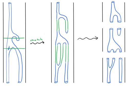
Consider the following sequence of holomorphic curves  given by
  . We see that away from
  , this is just converging to the curve
  . But near
  , if we reparametrize the domain by
  , we see this converges to the sphere
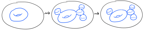
  . In this case, our curve formed what is often called a bubble. More generally, a curve can split off many bubbles at a time. For an example of this, consider instead
  given by
  , in which a new bubble forms at
  in addition to the one discussed above. More generally, a sequence of curves can limit to a curve with trees of bubbles sticking out.
Such bubble trees are called stable or nodal or cusp curves (or probably a lot of other things), depending upon how old your reference is and to whom you talk. The incredible theorem, which goes under the name of Gromov compactness, is that this is the only phenomenon which precludes a limit from existing. We state this vaguely as follows:
Theorem [Gromov ’85]: The moduli space of curves of energy bounded by some constant  (modulo reparametrization of domain) can be compactified by adding in stable curves of total energy bounded by .
Another generally important tool is that of the evaluation map. Suppose that we wish to study the moduli space of simple J-holomorphic maps  in the homology class . Suppose
  is the group of biholomorphisms of
  . Then the group
  acts on
  by
by  . Notice then that the evaluation map
  only depends on the orbit, and hence descends to a map
  . Proving enough properties of such an evaluation map sometimes allows us to compare the smooth topology of to that of . There are other variants of this – sometimes we wish to evaluate at multiple points, or sometimes we consider J-holomorphic discs and want to evaluate along boundary points. And often the evaluation map extends to the compactified moduli spaces considered above.
Finally, we come to dimension 4, where curves might actually generically intersect each other. With respect to these intersections, there are two key results to highlight. The first is positivity of intersection (due to Gromov and McDuff), which states that if any two J-holomorphic curves intersect, then the algebraic intersection number at each intersection point is positive (and precisely equal to 1 at transverse intersections). This can be thought of as some sort of rudimentary version of a so-called adjunction inequality (due to McDuff), which states that if  is a simple J-holomorphic curve representing the class
  with geometric self-intersection number
  , then
 .
.
Further, when is immersed and with transverse self-intersections, this is an equality, yielding an adjunction formula.
A first example – Fillable implies tight (in 3 dimensions)
On a first pass, I want to expand upon the example of fillability implying tightness in three dimensions which Roger Casals discussed in his introductory talk. Really, we prove the contrapositive – that an overtwisted contact manifold cannot be filled. For simplicity, we will consider exact fillings. This result is typically attributed to Gromov and Eliashberg, referencing Gromov’s ’85 paper as well as Eliashberg’s paper on filling by holomorphic discs from ’89. This is essentially the same proof in spirit, although we take a little bit of a cheat by considering exact fillings.
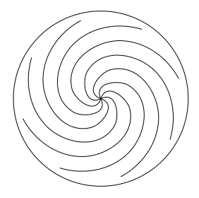
Firstly, recall that an overtwisted contact manifold  is one such that there exists an embedding of a disk
  , such that the so-called characteristic foliation
  on
on  , which is actually a singular foliation, looks like the following image, with one singular point in the center and a closed leaf as boundary.
So now suppose has an exact filling  . We study the space of certain J-holomorphic disks with boundary on the overtwisted disk. The key is that a neighborhood of the overtwisted disk
  actually has a canonical neighborhood in
  up to symplectomorphism, and one can pick an almost complex structure to be in a standard form in this neighborhood. It turns out that with this standard choice, in a close enough neighborhood of the singular point
  in the interior of , all somewhere injective J-holomorphic curves are precisely those living in a 1-parameter family, called the Bishop family, which radiate outwards from the singular point .
Let us be a bit more precise, so that we can see this Bishop family explictly. Consider the standard 3-sphere  , with its standard contact structure given by the complex tangencies, i.e.
 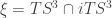 , with
  the standard complex structure on
  . Then consider the disk given by
  . The characteristic foliation on this disk looks like the characteristic foliation near the center of the overtwisted disk, so a neighborhood of this disk in
  yields a model for a neighborhood of the center of the overtwisted disk. We may assume the almost complex structure in this neighborhood is just given by the standard one, . Then the Bishop family is just the sequence of holomorphic disks given by
 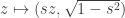 for
for  a real constant near 0. That these are all of the somewhere injective disks is a relatively easy exercise in analysis. Namely, suppose we had such a disk of the form
  . Then since boundary points are mapped to the overtwisted disk,
  . But each component of
  is harmonic, hence satisfies a maximum principle. Therefore,
  . But by holomorphicity, cannot have real rank 1 and so must be constant. Hence, any disk in consideration must have is a real constant.
All of these disks live in , but in particular in the slice where the second component  is real, so we can draw this situation in
  by forgetting the imaginary part of . This is depicted in the following figure.
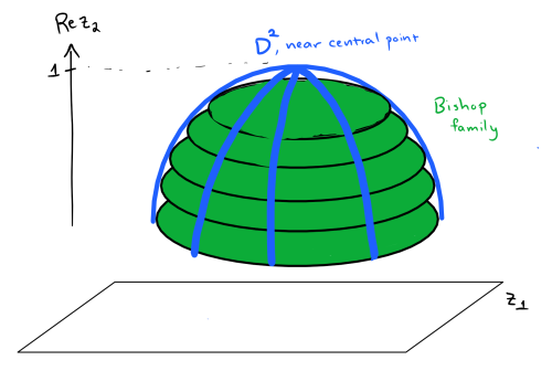
This Bishop family lives in some component of the moduli space of somewhere injective J-holomorphic disks with boundary on . Perturbing , one can assume this component is actually a smooth 1-dimensional manifold. We can compactify this moduli space by including stable maps, i.e. disks with bubbles, via Gromov compactness. On the Bishop family end, we see explicitly that the limit is just the constant disk at the point . So there must be another stable curve at the other boundary of this moduli space. We prove no such other stable curve can exist.
Similar to how we proved that the only disks completely contained in a neighborhood of the singular point on the overtwisted disk must have been part of the Bishop family, one can use a maximum principle argument to conclude that every holomorphic disk entering this neighborhood must have been in the Bishop family. Alternatively, one can use a modified version of positivity of intersections to conclude that continuing the moduli space away from the Bishop family, these boundaries have to continue radiating outward. Either way, the moduli space has to stay away from the central singularity of the overtwisted disk . But also, the boundary of a J-holomorphic disk cannot be tangent to  , and in particular cannot be tangent to
  . This is by a maximum principle which comes from analytic convexity properties of a filled contact manifold.
The only possible explanation is that this is a stable curve with some sphere bubble having formed in the interior of  . But one checks that the relation
  implies that for a -holomorphic sphere
  , we have
  . This vanishes by Stokes’ Theorem since
  is exact, and so must be constant, and so there is no bubble. In other words, this cannot explain the other boundary point of the component of the moduli space containing the Bishop family, so this yields a contradiction.
On McDuff’s The structure of ruled and rational symplectic 4-manifolds
Emily Maw’s talk from the workshop followed this paper by Dusa McDuff. In what follows, we shall consider triples  such that
  is a smooth closed symplectic 4-manifold and
  is a rational curve, by which we mean a symplectically embedded
  . We call a rational curve exceptional if
  with respect to the intersection product on
  (with respect to its orientation coming from ). We say is minimal if
  contains no exceptional curves. The main theorem is as follows:
Theorem [McDuff ’90]: If is minimal and  , then is symplectomorphic to either:
 , in which case is either a complex line or a quadric (up to symplectomorphism).
- A symplectic -bundle over a compact manifold , in which case is either a fiber or a section (up to symplectomorphism).
Before describing the proof, which is the part involving J-holomorphic curve techniques, we apply this to strong fillings. We shall concern ourselves with fillings of the lens spaces  with their standard contact structures, where
  is an integer. Let us first define this contact structure. Recall that the standard contact structure on
  is the one coming from complex tangencies by viewing . Then the standard contact structure on is the one given by the quotient
  where the action of
  given by
  preserves the contact structure, so that it descends.
Theorem [McDuff ’90]: The lens spaces all have minimal symplectic fillings  , and when
  , these fillings are unique up to diffeomorphism, and further up to symplectomorphism upon fixing the cohomology class
 ![[\omega]](https://s0.wp.com/latex.php?latex=%5B%5Comega%5D&bg=ffffff&fg=333333&s=0&c=20201002) . The space
. The space  has two nondiffeomorphic minimal fillings.
Proof (sketch): The complex line bundle  over comes with a natural symplectic structure, and this forms a cap for . The zero section of is a rational curve of self intersection . McDuff’s explicit classification includes examples
  for any such given , and thus gives a minimal filling for . The remaining statements come from a more detailed analysis of the classification result.
Now, I will not go through all of the details of McDuff’s proof of the main theorem, but I will highlight where various J-holomorphic tools appear in the proof. Let me break up the proof into two big pieces.
Step 1: “Mega-Lemma” Consider minimal as above. There is a tame almost complex structure such that ![[C]](https://s0.wp.com/latex.php?latex=%5BC%5D&bg=ffffff&fg=333333&s=0&c=20201002) can be represented by a -holomorphic stable curve of the form
can be represented by a -holomorphic stable curve of the form  , where:
- Each
![A_i := [S_i]](https://s0.wp.com/latex.php?latex=A_i+%3A%3D+%5BS_i%5D&bg=ffffff&fg=333333&s=0&c=20201002) is -indecomposable (meaning any stable curve representing
is -indecomposable (meaning any stable curve representing  must actually be a legitimate curve of one component)
- The almost complex structure is regular for all curves in the class .
- The
 are distinct and embedded curves of self-intersection -1, 0, or 1, with at least one index for which
  .
.
We didn’t prove this at the workshop, so I won’t discuss it in detail here. But this is a major reduction into cases. For example, if  and
and  , then it had already been shown that this implies that
  . This bleeds into…
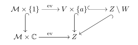
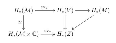
Step 2: Using the evaluation maps constructively
Let us discuss the proof of this last fact briefly. The idea is as follows. We consider the moduli space  consisting of simple holomorphic spheres representing the class
 ![A = [S]](https://s0.wp.com/latex.php?latex=A+%3D+%5BS%5D&bg=ffffff&fg=333333&s=0&c=20201002) . This comes with an evaluation map of the form
. This comes with an evaluation map of the form

where is the group of automorphisms of . Both sides have dimension 8 and this evaluation map is injective away from the diagonal since  and we have positivity of intersection. Therefore, this map has degree 1, and so any pair of distinct points on
  has a unique curve passing through it. This is enough to show .
Let us do another case, but show that the adjunction formula also comes into play.
Proposition: Suppose  is a simple homology class in (i.e. is not a multiple of another homology class) with
  , and suppose
  is a rational embedded sphere representing . Then there is a fibration
  with symplectic fibers and such that is one of the fibers.
Proof (sketch): The idea is to consider the moduli space  of rational embedded -holomorphic curves with 1 marked point
  , and where is chosen to tame and such that is itself a -holomorphic curve, and where we have quotiented by reparametrization of the domain. Then one can compute the dimension of this moduli space at a given curve in the appropriate way as
![d = \dim V + 2c_1(TV) \cdot [C] - 4](https://s0.wp.com/latex.php?latex=d+%3D+%5Cdim+V+%2B+2c_1%28TV%29+%5Ccdot+%5BC%5D+-+4&bg=ffffff&fg=333333&s=0&c=20201002) ,
,
where the last -4 comes from quotienting by the subgroup of  fixing the marked point. Applying adjunction for the curve represented by , so that
 ![[C] \cdot [C] = 0](https://s0.wp.com/latex.php?latex=%5BC%5D+%5Ccdot+%5BC%5D+%3D+0&bg=ffffff&fg=333333&s=0&c=20201002) , yields
, yields  . We also have an evaluation map

Since , there is at most one -curve through each point in , so it follows that this evaluation map has degree at most 1, and hence equal to 1 by regularity. This yields the structure of a fibration  where the fibers are precisely the curves in our moduli space. Since the fibers are holomorphic, they are symplectic by the taming condition.


is a compatible almost complex structure for


![((-\epsilon,0] \times M, d(e^t\alpha))](https://s0.wp.com/latex.php?latex=%28%28-%5Cepsilon%2C0%5D+%5Ctimes+M%2C+d%28e%5Et%5Calpha%29%29&bg=ffffff&fg=333333&s=0&c=20201002)


![\overline{\mathcal{M}_0} = [0,1] \times S^1](https://s0.wp.com/latex.php?latex=%5Coverline%7B%5Cmathcal%7BM%7D_0%7D+%3D+%5B0%2C1%5D+%5Ctimes+S%5E1&bg=ffffff&fg=333333&s=0&c=20201002)
![[0,1] \times S^1](https://s0.wp.com/latex.php?latex=%5B0%2C1%5D+%5Ctimes+S%5E1&bg=ffffff&fg=333333&s=0&c=20201002)


![([0,1] \times T^2, \cos(2\pi t)d\theta_1 + \sin(2\pi t)d\theta_2)](https://s0.wp.com/latex.php?latex=%28%5B0%2C1%5D+%5Ctimes+T%5E2%2C+%5Ccos%282%5Cpi+t%29d%5Ctheta_1+%2B+%5Csin%282%5Cpi+t%29d%5Ctheta_2%29&bg=ffffff&fg=333333&s=0&c=20201002)


for
via the isomorphism induced by inclusion
otherwise
, then all strong aspherical fillings of


where
is the standard radial Liouville vector field on
is modelled after the positive symplectization of


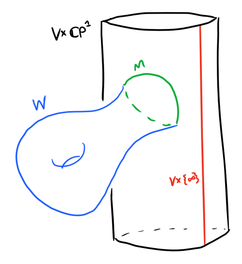


![[u] = [\{v\} \times \mathbb{C}P^1]](https://s0.wp.com/latex.php?latex=%5Bu%5D+%3D+%5B%5C%7Bv%5C%7D+%5Ctimes+%5Cmathbb%7BC%7DP%5E1%5D&bg=ffffff&fg=333333&s=0&c=20201002)


.
. First of all,


 has a structure group which can be reduced to
  , but the complex bordism group is well known to satisfy
  . As a consequence, every contact manifold is smoothly fillable. We must therefore consider fillability questions which extend beyond the realm of complex bordism in order to discover interesting phenomena.
 such that
  . There is a generalization in higher dimensions due to
  is
is  is strongly fillable if there is a weak filling
  such that one can find a Liouville vector field
  , such that
  gives a (properly cooriented) contact form for
  where
where  .
. on
on  and
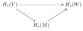
and  fits into an exact triangle with Morse homology, and so one can understand the topology of a filling from its symplectic homology. One might be interested, for example, in studying fillings with
  , in which case the homology of the filling is completely determined by