Contact Hamiltonians (Introduction)

This entry is part of the series of posts on the recent work of  M. S. Borman, Y. Eliashberg and E. Murphy on the existence and classification of overtwisted contact structures in all dimensions. In the previous two entries the construction in the 3–dimensional case and Gromov’s h–principle for the open case have been explained.

The essential fact in Eliashberg’s 3–dimensional argument (this is part 2, two entries ago) is the control on the characteristic foliation: the extension problem is reduced to being able to fill a 2–sphere with a contact ball given a particular characteristic foliation on the boundary. This can be done explicitly by deforming the local model provided by the standard overtwisted contact ball in order to have the given characteristic foliation on the boundary. The construction in higher dimensions is not quite the same and it relies on the use of contact Hamiltonians, hence this and subsequent entries. This first introductory entry should help the reader to follow the next entries, each entry should however be readable on its own.

Consider a contact manifold of dimension 2n+1. The information of a contact structure is contained in a 1–form (locally this is the data of 2n+1 functions, plus another one as a conformal factor, satisfying 1 non–degeneracy equation). This data can be drastically reduced when restricted to simple topological subsets if we choose appropriate coordinates: for instance, the Darboux theorem tells us that the normal form of a contact 1–form around a point is . It will be helpful for the reader to understand the geometric proof of the Darboux theorem, see Theorem 2 in Page 5 of Topological methods in 3-dimensional contact geometry. The strategy is finding a suitable flow to obtain the desired coordinates.

Suppose that we have a contact manifold and a codimension–1 distribution on the manifold such that it restricts to on each slice . In these hypotheses:

Lemma: There exists the following normal form for the 1–form , we can write for some smooth function .

Proof: Consider the product manifold as a trivial fibre bundle over the disk . The data in the hypothesis gives a connection in this bundle whose parallel transport is by contactomorphisms, it is defined as the skew–orthogonal complement of the symplectic subspace in the bundle with respect to the 2–form (which is not necessarily symplectic). We can then consider the radial vector field in the base and lift it to the total space . The pull–back of the contact form by this flow is (conformally) of the form for some function . The reason being that the radial factor cannot appear because in the trivializing coordinates (provided by the flow of the lift), the lift of the radial vector field belongs to the distribution.

There are a couple of technical details regarding the existence of the flow, which can be translated into the size of the base disk. Let us not focus on that. Thanks to the Lemma we have the following reduction of the extension problem.

Suppose that on a given almost contact (2n+1)–fold V we have a contact structure on all of V except on a neighbourhood of a codimension–2 submanifold M with trivial normal bundle. If the almost contact structure satisfies the hypothesis for the Lemma in , then the extension problem for the contact structure is reduced to:

Problem: Given a germ of a contact structure on described by a function , does there exist a contact structure on such that it restricts to the given germ on ?

There are two remarks at this point. First, the meaning of the function H is really geometric. It describes the angle of rotation of the contact structure in the radial direction, in particular the condition for to be a contact structure on reads (this is often stated as the contact structure has to rotate). Second, the extension does not need to be of the form , we just need a contact structure on .

Example 1 (Tight): Consider and the function . The contact form is and since the function H verifies the contact condition on this defines a contact structure on . This is the standard contact structure on the ball.

Example 2 (Overtwisted): Consider and . The contact form is then , which should be read as . This is the standard overtwisted contact structure on the ball if the radius of the disk is larger than .

This second example has the following very nice feature: the function is negative at r=2. This provides a solution to the problem of extending a germ in to the interior if this germ is everywhere negative. Although a priori it seems non–sense to go from 0 to a negative value growing (in order to preserve the contact condition) this can be done by inserting a pole, i.e. going to infinity (and then continuing from minus infinity). This phenomenon underlies many h–principles, try to solve for instance Section 4.1.1 from Chapter 4 in Eliashberg–Mishachev book.

The functions H appearing in the above constructions are called contact Hamiltonians.

Problem (Easy Case): Given a germ of a contact structure on described by a positive function , does there exist a contact structure on such that it restricts to the given germ on ?

Answer: Yes. In this case the extension can be a contact structure of the form where extends H and is such that . Certainly, we just need to construct a function which at the origin looks like and then it grows in the radial direction until we reach the value given by H on the boundary . The existence of such a function is immediate.

The difficult case is that of a germ of a contact structure defined by a Hamiltonian which is negative in some points and positive in others (the presence of such negativity requires overtwistedness). The situation described above is quite hard because we may not even understand the (contact) topology of M. The first step is to focus on a (2n-1)-ball, or star–shaped domain, in .

In the next entry, Contact Hamiltonians (Part I) we will continue to use contact Hamiltonians and relate them to Eliashberg’s 3–dimensional argument using the characteristic foliation. The essential word will be monodromy.

In the context above, monodromy arises as follows: consider the contact germ on and lift the vector field to the connection defined before. Its flow at time equal to the length of the circle (say 1) defines a contactomorphism of the fibre . This is the monodromy contactomorphism.

There is however another way to obtain a contactomorphism of if we have a  function (referred to as a time–dependent contact Hamiltonian). Indeed, compute the Hamiltonian contact vector field X associated to H, which is the unique solution of

and

where is the Reeb vector field. Then the time–1 flow of the Hamiltonian vector field is a contactomorphism of M. This contactomorphism is said to be generated by the contact Hamiltonian H.

Lemma: Given the contact germ on , the monodromy contactomorphism coincides with the contactomorphism generated by H.

The proof of this lemma is a nice exercise on linear algebra using the defining equation of the connection. This setup can be explicitly studied in 3–dimensions where the monodromies (and the functions H) can be drawn and they correspond to ODEs in the plane. In the next post we will proof Eliashberg’s theorem in dimension 3 from the contact Hamiltonian perspective.

Gromov’s h-principle for open contact manifolds

Continuing towards a discussion of the proof of existence and classification of overtwisted contact structures in higher dimensions, here I want to talk about h-principles, and contact structures on open manifolds.

h-principles

Given a partial differential equation or partial differential relation (like the contact condition ), one can formally replace the derivatives of the variables with independent formal variables (i.e. for a 2-form ). Solving this new problem where the derivatives are replaced by independent formal variables is purely an algebraic topology problem. If the algebraic topology problem has no solution then certainly the partial differential relation has no solution. However, it is generally surprising when the converse holds: namely, the existence of a solution to the algebraic problem implies the existence of a solution of the partial differential relation. A theorem that proves this type of statement is referred to as an h-principle.

The language of jet bundles and holonomic sections will help make this more precise below.

The main results of Borman, Eliashberg, and Murphy that we are heading towards are an h-principle for contact and almost contact structures on higher dimensional closed manifolds which says that any almost contact structure is homotopic through almost contact structures to an actual (overtwisted) contact structure, and a parametric version of this h-principle which says that any family of almost contact structures connecting two genuine overtwisted contact structures can be homotoped to a family of genuine contact structures connecting the fixed overtwisted contact structures on the ends.

While contact structures on closed manifolds can have incredibly complicated classifications (because of the rigidity of tight contact structures), it is a result of Gromov that on open manifolds the geometric subtlety disappears and the classification of contact structures is reduced to algebraic topology by an h-principle. This post is based on a talk given by Kyler as part of the discussion of the proof of flexibility of overtwisted contact structures in higher dimensions, though the original source for the content is Gromov’s Partial Differential Relations book.

Define a (cooriented) almost contact structure on an odd dimensional manifold to be a cooriented hyperplane distribution, together with a non-degenerate 2-form on the distribution. In dimension 3, this is homotopy equivalent to the space of co-oriented 2-plane distributions. Gromov’s theorem is:

Let V be an open manifold. Then the inclusion of cooriented contact structures on V into cooriented almost contact structures on V is a homotopy equivalence.

The proof is based on two main ideas: the holonomic approximation theorem on neighborhoods of codimension one polyhedra, and the fact that all open smooth manifolds smoothly retract onto a neighborhood of a complex of codimension at least one. I’ll start with the former.

The 1-jet space of a fiber bundle , is a bundle where the fiber over consists of sections of X defined over a neighborhood of p up to an equivalence which equates sections that agree up to 1st order near p. (The r-jet bundle is defined similarly where you equate sections which agree up to rth order, but here we will only need the 1-jet bundle.) A section of chooses an equivalence class of sections over each point in : for each , where is a point in the fiber , and specifies the first partial derivatives of a function at that point. However, even though the section is smooth, need not specify the actual derivative of since is encoded as an independent direction in the fibers of . A holonomic section of a 1-jet space is one where this linear variation specified by agrees with the actual partial derivatives of the differentiable section of given by the 0th order information of the section. The holonomic approximation theorem aims to approximate an arbitrary section of the 1-jet bundle by a holonomic section as well as possible.

Here the blue curve represents a section of . The grey curve represents its projection to the 0th order information, and the 1st order information is encoded in the dimension coming out of the page. Representing the value the blue curve takes in this dimension by a green line of the appropriate slope centered at each point on the grey curve, we see that this is not a holonomic section because the 1st order information is not tangent to the curve.

The important relevant example for Gromov’s theorem is when , so sections of the bundle are 1-forms. Sections of the 1-jet space keep track of two coordinates: the pointwise values of the underlying 1-form and its formal linear variation. Locally, is a trivial bundle, and a section is just the graph of a function on . Modding out by the equivalence relation, we get that for a section , keeps track of the point , a point in and an n by n matrix at that point which specifies the formal first partial derivatives of a graph in that equivalence class (where n is the dimension of V). Symmetrizing this matrix (), gives the coefficients for a 2-form. When the section of is a holonomic section, this 2-form built from the 1st order information of the section, is the exterior derivative of the 1-form which gives the 0th order information of the section. Given any pair of a 1-form and a 2-form, there is a section of such that the 0th order information gives and after symmetrizing the 1st order information we get . For holonomic sections, this process gives a pair where is a 1-form.

There are certain limitations on the extent to which we can approximate an arbitrary section by a holonomic one. For example if we consider the 1-jet space of the bundle . A section of the 1-jet space is given by specifying the pointwise data and a formal 1st derivative. An example of a section has pointwise data given by the graph of , and formal derivative specified as 0 (horizontal lines at each point). To approximate this by a holonomic section, we would need to find a function g whose pointwise values only differ from those of by , and whose derivative only differs from zero by . Such a function would contradict the mean value theorem. So we cannot hope to approximate an arbitrary section by a holonomic one at every point. On the other hand, we can approximate the section in a small neighborhood of a point.

This motivates the idea to look at codimension 1 subspaces. Taking the previous example and just taking the product with a trivial extra dimension with coordinate y, we run into the same problem: that if we can only move up with a tiny slope in the x-direction, we cannot get up far enough by just moving along a path that has slope 1 in the x direction and does not move in the y-direction. However if we are allowed to perturb the path to lengthen it in the extra y-dimension that we have by adding many zig-zags, then we can do this approximation.

Moving along the black curve, there is no holonomic approximation which stays close to the horizontal planes. However, moving along the perturbed red curve, we can find a closer approximation which is holonomic.

This leads us to the precise theorem:

Holonomic approximation theorem: Let be a polyhedrong of codimension at least 1 and suppose we have a section of the jet bundle defined over a neighborhood of A. Then for any , there is a small isotopy of A (measured in the topology), and a holonomic section defined in a smaller neighborhood of which is close to the chosen section.

Suppose we have an almost contact structure on the open manifold V of dimension n. In order to use this theorem to prove Gromov’s theorem, we must identify a good codimension 1 subset of our open manifold V, where we can use holonomic approximation to find a genuine contact structure on a neighborhood of this subset which is close to the almost contact structure we are considering. Choose a triangulation of V, and for each top dimensional simplex, choose a path from the barycenter of that simplex out to infinity which avoids the barycenters of other simplices. The parts of the 2-skeleton which do not intersect these paths form a codimension 1 subcomplex S. The entire manifold smoothly deformation retracts onto arbitrarily small neighborhoods of S.

Now apply the holonomic approximation theorem to the pair (which corresponds to a section of ) along S. Then on a tiny perturbation of S, there is an actual holonomic section corresponding to which is very close to . By choosing our sufficiently small so that and are sufficiently close, we can ensure that the straight line homotopy between them stays in the space of almost contact structures (since the almost contact condition is an open condition (). Therefore the holonomic approximation theorem implies we can homotope our almost contact structure to be contact on a neighborhood of the perturbed S.

Observe that if is the end of the deformation retraction which sends V into the neighborhood of S where the almost contact structure is now genuinely contact, then pulls back the almost contact structure on V to a genuine contact structure on V. The deformation retraction provides a homotopy between the almost contact structure which is contact on the neighborhood of S to the genuine contact structure coming from this pullback. Therefore concatenating the homotopy provided by the holonomic approximation theorem with the homotopy provided by the deformation retract, gives a homotopy from our original almost contact structure to an actual contact structure on V.

Classifying Overtwisted contact 3-manifolds

Eliashberg proved that overtwisted contact structures up to isotopy are classified by their homotopy class in the space of 2-plane distributions in a 1989 paper. The higher dimensional case shares some similar structural aspects to the proof in 3 dimensions, so it seems worth going through the original result. I will try to mention the relations with the higher dimensional proof throughout. My sources here are Eliashberg’s original paper (Inventiones 1989), and the explanation of the proof in Geiges’ Introduction to Contact Topology book in section 4.7.

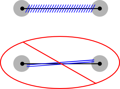
Starting at the beginning: an overtwisted disk in a contact 3-manifold is an embedding of the disk where the contact structure on is the kernel of . In dimension 3, we can alternatively define an overtwisted disk as an embedded disk whose boundary is Legendrian (tangent to the contact planes), such that the framing given by the contact planes agrees with the framing given by the surface. The existence of an overtwisted disk by one definition implies the existence of an overtwisted disk by the other definition, so we say a contact structure is overtwisted if it contains an overtwisted disk (using either definition).

The main idea is to start with a distribution, and homotope it piece by piece until it becomes a contact structure on the entire manifold. In order to extend the contact structure over the entire manifold, the existence of overtwisted disks is needed. This shows that every homotopy class contains a contact structure. In dimension 3 this followed from the work of Martinet who constructed a contact structure on each 3-manifold with surgery techniques and that of Lutz who showed that you can use Lutz twisting to modify the homotopy class of the contact structure however you want to without changing the 3-manifold. To show that any two overtwisted contact structures and which are homotopic are isotopic uses a parametric version of the extension construction. The homotopy between them gives an interpolating interval family of 2-plane distributions , and using the same ideas, we can homotope the intermediate distributions piece by piece until they become a smooth family of actual contact structures interpolating between and . Then by Gray’s theorem and are contact isotopic.

Note: everything here can be done relative to a closed subset; namely, if the 2-plane distribution is already contact on an open neighborhood of a closed subset, the homotopies can be chosen to fix the 2-plane distribution on that closed subset. This is in fact necessary to preserve the existence of the overtwisted disk throughout the modifications of the distribution, and to preserve the contact structures which are the end points of a 1-parameter family of distributions.

In fact the parametric version of the proof can be done when the parameter space is any compact set, so this can be used to show a more general statement. Let denote the space of overtwisted contact structures on M with a fixed overtwisted disk, and let denote the space of 2-plane distributions which also contain the fixed overtwisted disk. Then the inclusion is a homotopy equivalence. (Technically, the parametric version shows that this is a weak homotopy equivalence, but the spaces are CW complexes so the Whitehead theorem implies it is a full homotopy equivalence.) The idea to reprove the extension theorem in a parametric version is also used in the higher dimensional proof.

Now for the argument that we can homotope the distributions to genuine contact structures piece by piece (while fixing the pieces that we like already). We start with a triangulation of the manifold. We will make the distribution contact first in a neighborhood of the vertices, and then in a neighborhood of the 2-skeleton in a controlled manner, so that it will extend over the 3-cells at the end. The overtwisted disks needs to show up on the boundary of the ball that needs to be filled in at the end, so the 3-cells are all connected together with tubes and then connected to a neighborhood of the overtwisted disk. The contact condition in dimension 3 geometrically indicates whether the planes are twisting at the correct speed in the correct direction determined by the orientations. Over neighborhoods of vertices, we can easily homotope the planes to twist as much as necessary. Then we need to ensure that the planes form a contact structure over a neighborhood of the 2-skeleton, and moreover, we need to control what the contact structure looks like on the remaining boundary spheres of the 3-cells. The way to keep track of this is through the characteristic foliations.

Characteristic foliations in dimension 3 and higher

Given a surface in a contact 3-manifold, the intersection of the contact planes with the tangent planes to the surface produces a 1-dimensional singular foliation of the surface called the characteristic foliation. Equivalently, we can look at the restrictions and to the surface, and define a foliation by the vector field defined by . Notice that such a vector field is necessarily in the kernel of the contact form, and is identically zero exactly when the contact planes are tangent to the surface (since then and is an area form). In higher dimensions, the intersection of the contact planes with the tangent planes no longer forms an integrable distribution, but there is still a 1-dimensional singular characteristic foliation defined via the contact form in the same way. However, the characteristic foliation in higher dimensions can look considerably more complicated, and controlling its behavior takes a few additional steps than what is needed for the 3-dimensional proof.

The characteristic foliations that we will aim for on the 2-spheres are as follows. First we want the foliation to be simple meaning it has exactly two singular points, one a source (the “north pole”) and the other a sink (the “south pole”), and all the limit cycles (closed orbits) are isolated. These limit cycles necessarily form parallels between the two poles. If additionally there is a curve running from the south pole to the north pole which is positively transverse to all of the (oriented) leaves of the foliation, then the foliation is called almost horizontal. This condition is met when all of the limit cycles are oriented from east to west when viewing the sphere as a globe and the limit cycles as lines of longitude. The benefit of the almost horizontal condition, is that the foliation is determined up to homeomorphism by a monodromy map from the interval to itself where the interval is the transverse curve, and the holonomy map is determined by flowing around the characteristic foliation once. The limit cycles correspond to fixed points of the holonomy. In the 2n+1 dimensional case, the monodromy will be a map from the 2n-1 disk to itself. In the 3-dimensional case, the homeomorphism type of the foliation is determined completely by whether the points are moved up or down the interval by the holonomy between each pair of fixed points. This is important because of the following lemma:

Lemma: Let be a contact structure defined near the boundary of a 3-ball. The question of whether extends over the ball depends only on the topological type of the characteristic foliation induced on the boundary sphere.

To prove the lemma, given two characteristic foliations on the sphere that are topologically equivalent, first identify the poles and limit cycles. Then show that in a small neighborhood of the boundary sphere which one of the characteristic foliations, there is another sphere which realizes the other characteristic foliation. Therefore, if the contact structure extends over the ball for the first foliation, it extends over the ball for the second.

Now we want to prove two things:
1. We can homotope the 2-plane field over a neighborhood of the 2-skeleton so that it is contact there and it induces almost horizontal characteristic foliations on the spheres which bound the remaining finitely many holes where the distribution may not yet be contact (inside the 3-cells).
2. Given a contact structure on the manifold in the complement of a collection of finitely many balls, such that the characteristic foliations are almost horizontal, and such that the contact structure contains an overtwisted disk, the balls can be connected together to each other and to the overtwisted disk so that the contact structure in a neighborhood of the resulting boundary sphere can be extended inside the resulting ball to a contact structure.

Part 1: Over the 2-skeleton, the failure of the 2-plane distribution to be contact amounts to the planes not twisting positively enough. However, we need to identify which direction we need to twist along. For this we find an auxiliary 2-dimensional foliation defined near the 2-skeleton (maybe not necessarily defined near the 0-skeleton) which is everywhere transverse to , and is parallel to the 1-simplices (each 1 simplex is contained in a leaf), and is perpendicular to the 2-simplices. Now consider the characteristic foliation determined by on each leaf of this auxiliary foliation. The characteristic foliation is nonsingular by the transversality condition, so we can cover this neighborhood of the 2-skeleton by pieces which can be identified with a subset of with 1-dimensional foliation given by curves parallel to the y-axis. By ensuring that the 2-planes twist enough along the leaves of this 1-dimensional foliation, we can identify each of these pieces of manifold together with the 2-plane distribution with a piece of . The idea is to twist along these “Legendrian curves” in a neighborhood of each simplex one by one, in a relative way so that we fix the parts that we have already made contact. The thing we want to avoid is at some point, one of the Legendrian curves may have two ends in the relative piece that we have already made contact and do not want to mess up. In order to avoid this, keep very close track of the angles between and the simplices and the angles between different adjacent simplices.

A question: why is the 2-dimensional foliation chosen parallel to the 1-simplices and perpendicular to the 2-simplices? Some thoughts: this might be needed to make the Legendrian foliation consistent from the neigbhorhood of the 1-simplices to the neighborhood of the 2-simplices, or it might be needed for the Legendrian foliation to accurately capture the angle the contact planes make with the simplices.

In the parametric case where we want to keep track of the angles of a family of distributions , we simply subdivide the compact parameter space into sufficiently small pieces so that the angles between the contact planes at a fixed point but at different times in the parameter space remain sufficiently small relative to the chosen simplicial complex. Then one can make a homotopy through contact structures for t in each subinterval, and by doing everything relative to the end points, this will gradually extend across the entire parametrizing interval.

The precise details of the argument are in Geiges’ exposition, but without getting bogged down in notation, here is the idea of the angle tracking argument. First choose a very fine simplicial complex where the maximal diameter, d, of the simplices becomes very small, but the angles between simplices remains bounded above by , and the minimum distance between disjoint simplices is less than some fixed constant multiplied by d. On each simplex, the amount that the angles of the contact planes change relative to each other is measured by a Gauss map from the simplex to . This change can be captured by a norm, which by choosing a good enough simplicial subdivision, can be assumed to be small relative to , so that across each simplex, the angle of the contact planes only changes by a very small fraction of .

Eliashberg defines “special simplices” as 1- or 2-simplices which contain some point p at which makes an angle less than with the simplex. The other 1- and 2-simplices are considered non-special. The idea of the special simplices is that the Legendrian curves which tell you which direction to twist in, make a small angle with the simplices, whereas with the non-special simplices, the Legendrian curves are “sufficiently transverse” to the simplices that the curves will have at least one end in the 3-simplices, away from the neighborhoods of the 0-, 1-, and 2-simplices where we may have already modified to be contact. By carefully keeping track of the angles between simplices and , and between at one point versus another (using the small norm assumption from the previous paragraph), one can show with triangle inequalities that if two special simplices were adjacent, the angle between them would be less than , which is not possible. Therefore the special simplices are isolated from each other, so we will perturb the distribution to become contact along the special simplices first and not worry about whether this changes the plane field near the other adjacent simplices as we will fix them later. Once this is done, we assume that we have modified to be contact in a neighborhood of all special simplices, and in a neighborhood of any 0-simplices (vertices) which are disjoint from the special simplices. The sizes of these neighborhoods are chosen relative to the constants and . Next modify the contact structure in small neighborhoods of the non-special 1-simplices (which are not the boundary of a special 2-simplex) rel boundary (where the structure is already contact and we don’t want to modify it anymore). The angle between the non-special simplices and the Legendrian foliation curves defined by is at least at each point. By having chosen the neighborhoods of the special simplices and 0-simplices small in terms of and the minimal distance between disjoint simplices, , we can ensure that none of the Legendrian curves through the non-special simplex hit the already contact neighborhoods in more than one end so we can twist the planes towards the end where we do not need to fix the planes.

In this picture the blue curves represent the “Legendrian foliation.” The black is the non-special 1-simplex, and the grey regions are where the 2-planes have already been perturbed to be contact.

Finally, we homotope the planes in a neighborhood of the non-special 2-simplices rel boundary (since the planes are contact over the entire 1-skeleton now). Again having chosen the previous neighborhoods sufficiently small in terms of , we can ensure that the Legendrian curves through these 2-simplices only intersect the neighborhood of the special and 1-simplices at one end so we can twist towards the free end.

A note about homotoping relative to a fixed closed subset: During this process, we modify the planes to be contact in certain areas and then freeze the planes there as we homotope the planes in other regions. In a similar way, if our planes were already contact in a certain region that we wanted to keep fixed from the beginning (e.g. a neighborhood of an overtwisted disk), we can do this. We just need to refine the simplicial subdivision enough near this relative set, so that we never get Legendrian curves with two ends inside the relative set.

Now we have reached a distribution which is contact in a neighborhood of the 2-skeleton, and thus in the complement of finitely many balls. We need to slightly enlargen these balls into the neighborhood of the 2-skeleton but without hitting the 2-skeleton, so that the balls are sufficiently round (they have normal curvatures bounded below by a positive constant). We can also assume some genericity of the contact structure on the boundary sphere within the roundness constraint. This together with the restrictions on the norm of the contact structure (it the planes can only twist a little bit over any simplex), ensures that the characteristic foliations on the boundaries of these enlargened balls are almost horizontal. The idea is to compare the Gauss maps along the boundary sphere of the tangent planes and the contact planes. If the characteristic foliation were not almost horizontal, the two Gauss maps, which agree at the positive singular point, would at some point become far apart (separated by angle ), which cannot happen in these tiny simplices where does not change its angle much.

Before going on to part 2, I want to briefly mention that in the higher dimensional version there is a part of the argument which involves keeping track of the angles of the hyperplanes relative to a foliation. There is again a distinction between pieces where the angles are sufficiently large and those that are relatively small. However, controlling the angles gets to a contact structure in the complement of balls (with a “saucer” type almost contact structure) but they do not have a sufficiently controlled characteristic foliation to fill in directly without a number of additional steps.

Part 2: At this point we have a finite set of balls in our manifold. The planes of have been homotoped to be contact in the complement of the interiors of these balls, and we have almost horizontal characteristic foliations on the boundaries. Furthermore, based on our original assumption, somewhere in the contact region is a neighborhood of an overtwisted disk, which we have fixed throughout, homotoping everything else relative to this piece. We will need to connect the almost horizontal balls to the overtwisted ball in order to fill them in. We first connect the finitely many almost horizontal balls to each other, by ordering them and then choosing a path from the north pole of one almost horizontal sphere to the south pole of the next. The connect sum of these spheres appears as the boundary of the balls together with a tiny neighborhood of the connecting path.

Note: if there is a closed set where we want to keep the contact planes fixed, we should choose our connect sum paths to avoid this set since we will modify the planes on the interior of the connected up ball.

The resulting characteristic foliation on the connect sum of all the almost horizontal spheres and the boundary of the neighborhood of the overtwisted disk is a simple foliation where there are two limit cycles oriented east to west (coming from the neighborhood of the overtwisted disk), and the rest of the limit cycles are oriented west to east (coming from the almost horizontal foliations). The standard overtwisted ball of radius in can be isotoped to a ball with boundary whose characteristic foliation is topologically equivalent to this connect sum. By the lemma mentioned before part 1, this is enough to fill in the holes. To see this isotopy consider the surfaces of revolution of smooth curves around the z-axis in in . Every time the curve intersects the line , we obtain an extra limit cycle. The orientation of the limit cycle (east to west or west to east) is determined as follows. The characteristic foliation is generated by a vector field defined by $laetx \iota_X\Omega=\alpha$ (where is restricted to the surface and is a positive area form on the surface). Therefore if we pair with a vector in the tangent plane to the surface which has a positive Reeb component, we obtain a positively oriented basis for the surface. The sphere surface is oriented as the boundary of the ball, so the outward normal to the sphere, followed by $X$ followed by a vector with a positive Reeb component forms a positive basis for . The Reeb vector field coorients the tangent planes, and points in the negative z direction at , so vectors with a negative z component have a positive Reeb component.

In this picture, the red vectors lie in the plane and are outward normals to the surface of revolution. The vector field generating the characteristic foliation on the limit cycles are pointing either directly in or out of the plane as indicated by the blue words. The green vector fields each have a negative z component and thus have a positive Reeb component. Observe that red, blue, green gives a positive basis for at each of these points. Furthermore notice that each limit cycle oriented by blue going out is moving east to west (there are two of these), and each limit cycle oriented by glue going in is moving west to east so we can create any number of these by creating intersections of the curve with on the “inside” of the curve. To make an odd number of limit cycles, have the curve intersect at a tangency on the inside.

This completes the 3-dimensional argument to homotope 2-plane fields containing an overtwisted disk to a contact structure. By doing this for an interval family of contact structures rel end points, we get that a family of overtwisted 2-plane fields can be homotoped to an isotopy of overtwisted contact structures.

Step 2 in the higher dimensional proof of Borman, Eliashberg and Murphy is somewhat different. First of all, one needs to establish more clearly what the necessary boundary structure of the balls is through an explicit model. The amount of flexibility in this model is not quite as much as the topological equivalence of characteristic foliations on spheres. Once the boundary model is established, each of the spheres is connect-summed to a neighborhood of an overtwisted disk (though they are not connected summed to each other, instead a bunch of copies of overtwisted disks are used, one for each hole). Then, using some contactomorphisms and various lemmas, it is possible to show that these connect sums of holes which have model contact structures on their boundaries with neighborhoods of overtwisted disks can be filled in with a contact ball. The filling of the holes is not as explicit as the surface of rotation model above in the 3-dimensional case. More on the higher dimensional case coming in later posts.

Overtwisted contact structures and h-principles

Twenty-five years ago Eliashberg established a dichotomy of contact structures on 3-manifolds as either tight or overtwisted. The overtwisted manifolds were motivated by the property that they satisfy certain flexibility principals. 1. Every co-oriented 2-plane field on a 3-manifold is homotopic to an overtwisted contact structure. 2. Any two overtwisted contact structures which are homotopic as 2-plane fields are isotopic as contact structures. (More generally, there is a homotopy equivalence between the space of contact structures and the space of 2-plane fields when you restrict each space to only include those with a particular overtwisted disk.) Recently, this theorem has been generalized to higher dimensions by Borman, Eliashberg, and Murphy , who explained their work at a recent workshop. The next few posts will be an attempt to share the intuition they gave, to work through some of the steps of their paper, to provide some historical background, and to discuss some related constructions and interesting open questions.

I also want to mention, that we are happy to give author permissions to young mathematicians who want to contribute blog posts. Thanks to Roger for agreeing to contribute on this topic, and welcome to the blog.

Graduate Student Topology and Geometry Conference

The 12th annual graduate student topology and geometry conference will be at UT Austin this April. The registration deadline is coming up on February 1. The website for registration and more information is http://ma.utexas.edu/conferences/gstgc14/. Many of the talks are given by graduate student participants, and we have lots of interesting faculty speakers in a range of topology/geometry topics. I encourage all grad students to register and submit a talk proposal (expository or original research).

Quick note: “A symplectic prolegomenon”

I just want to draw your attention to a survey that appeared on the arXiv on January 1: A symplectic prolegomenon, by Ivan Smith.  The main point is to motivate and illustrate the Fukaya category, and to show how its algebraic structures amplify the power of Floer cohomology.  Smith uses the running examples of the nearby Lagrangian conjecture and the symplectic mapping class group to demonstrate these algebraic structures (the Oh spectral sequence, the exact triangle associated to a Dehn twist, …) in action.  There are lots of applications throughout, and one nice feature is that section 5 consists of explicit descriptions of the Fukaya categories of six (families of) symplectic manifolds.

So it’s great winter break reading, check it out!  It collects together a lot of information that had previously been scattered over a bunch of different papers.  And it includes the take-home messages of a number of rather intimidating papers.

Seiberg Witten 4: Moduli spaces and invariants

This is my last post on defining the Seiberg-Witten equations and invariants for closed 4-manifolds based on a learning seminar at UT. Maybe I’ll post about some applications later on.

The Seiberg-Witten Configuration Space

We start with a Riemannian 4-manifold (M,g) and a Spinc structure on M. As we have seen, this data gives rise to the associated bundle and the determinant line bundle .

Let be the set of all Hermitian connections on . We have seen that such a connection gives rise to a connection on which is compatible with the Clifford multiplication.

The Seiberg-Witten configuration space is defined as

The Seiberg-Witten equations

The Seiberg-Witten equations take an element as their input. We are now prepared to define these equations.

As discussed in an earlier post, a connection A on gives rise to a connection on . Note that for , so . Therefore we have a Clifford structure

which composes with the connection

to get a Dirac operator

Denote the curvature of the connection A by . Then the curvature is a matrix of 2-forms on M, so we can consider its self-dual and anti-self dual parts and .

Let denote the traceless part of the endomorphism .

Now we can define the (perturbed) Seiberg-Witten equations. Fix a closed 2-form (the pertubation parameter). Then the Seiberg-Witten equations are:

The input to these equations is an element . The elements of which are solutions to these equations are called (-)monopoles.

The Gauge Action

The gauge group is . It acts on by

While it seems natural enough to act on the section by multiplication, why do we define the action ? Specifically where is the 2 coming from?

A is the connection of the determinant line bundle L of . We would really like to think of the gauge group as acting on . If acts on by multiplication , then the induced action on is multiplication by . (This goes back to the fact that in coordinate charts, the spinc structure is obtained by tensoring the spin structure with the square root of the determinant line bundle L.) Now we can look at how this acts on the covariant differentiation induced by the connection A on L. Here the natural action is conjugation

For we can consider its stabilizer in . If the stabilizer of C is trivial, we say C is irreducible, otherwise we say C is reducible. It is easy to show that the reducible elements are exactly those with , and that their stabilizers are the constant maps into .

The Seiberg-Witten moduli space

The Seiberg-Witten solution space is the space of elements for which the Seiberg-Witten equations are satisfied. To obtain the moduli space from this, we want to mod out by the gauge action. In order for this to be well defined, we first need to check that the space is invariant under the gauge action.

For the first equation, we can prove that because and because we can think locally that so taking its exterior derivative gives 0. Furthermore , so the first equation is invariant under the gauge action.

For the second equation, can be understood by breaking up the dirac operator into the composition of the Clifford multiplication and the connection on .

The discussion above about why the gauge group acts as it does on A is related to the fact that . Applying the Clifford multiplication to this connection acting on and using the Leibniz rule for connections eventually simplifies to show that so the solutions to are invariant under the gauge action.

Therefore we can mod out the Seiberg Witten solution space by the gauge action to get a well-defined space.

Properties of the Seiberg Witten moduli space

The reason the Seiberg-Witten equations are so useful is that the moduli space is actually a compact smooth manifold in many cases. When there are no reducible solutions to the equations, the moduli space defined by a generic perturbation is a smooth manifold (one needs to show that the linearization of a map defined by the Seiberg Witten equations and the gauge action is Fredholm and then use Sard-Smale to show that generic perturbations correspond to regular values).

Compactness of the manifold requires some analytic estimates. The Weitzenbock forumla is the main tool in obtaining bounds on solutions to the Seiberg-Witten equations.

After going through hard work to show these properties, which I am avoiding here, one just needs to worry about reducible solutions. Notice that if there are reducible solutions then they satisfy for our chosen perturbation. Since both of these forms are closed, they represent cohomology classes. The cohomology class of the curvature is independent of A, so we only have reducible solutions when . When the dimension of the positive second homology is at least 1, then a generic perturbation will avoid this phenomenon.

The Seiberg-Witten invariant of a 4-manifold is given by the homology class of the moduli space of solutions in the configuration space. This configuration space is homotopy equivalent to so its cohomology has a canonical generator in even degrees. By evaluating this generator against the homology class of the Seiberg-Witten moduli space we obtain an integer .

A priori this integer depends on the metric and perturbation, but when , the subspace of perturbations which allows for reducible solutions (bad perturbations) is codimension 2. Since the space of metrics on a manifold is convex, we can find a path through the space of metrics and good perturbations connecting any two pairs which lifts to a cobordism between the moduli space at and the moduli space at . Therefore SW gives a diffeomorphism invariant of the 4-manifold, and it has been used very effectively to distinguish many homeomorphic but not diffeomorphic 4-manifolds (exotic pairs).

When , there is a codimension 1 space of bad perturbations which forms a wall between two chambers. Within each chamber stays constant, and there is a well-understood wall-crossing formula describing the difference of SW in the two different chambers. By keeping track of a little more information, it is still possible to use information from the Seiberg-Witten invariants to distinguish exotic pairs (this has been used a lot for finding exotic ).

Seiberg Witten 3: Dirac operators, Spin and Spinc connections

This is my third post on the set-up for the Seiberg-Witten invariants of 4-manifolds. The next post will finally define the Seiberg-Witten equations and invariants, so this is the last bit of background.

Symbols, generalized Laplacians, and Dirac operators

In order to define the Seiberg-Witten equations, we need to understand certain partial differential operators called Dirac operators. If you don’t know the formal definition of partial differential operators and their symbols, here is a link with some definitions and examples.

The class of all second order partial differential operator with the same symbol as the usual Laplacian: are called generalized Laplacians. Note that the symbol of a generalized Laplacian is an isomorphism on each fiber for , which means generalized Laplacians are elliptic operators. An elliptic operator L is good because there are estimates on the norms of solutions to equations of the form . This allows us to use Fredholm theory to describe the space of solutions to equations using elliptic operators. (In particular the linearization of an elliptic operator is Fredholm, i.e. has finite dimensional kernel and cokernel).

Dirac operators are 1st order partial differential operators which square to a generalized Laplacian. Dirac operators inherit many of the nice properties of Laplacians, specifically they are also elliptic (though in a weaker sense than the Laplacian–my vague understanding is that the bounds we get from ellipticity of the Laplacian are uniform, whereas the bounds we get from ellipticity of a Dirac operator depend on the point in the manifold; in the case of compact manifolds these coincide).

Dirac Operators and Clifford multiplication

We mentioned above that the symbol of a generalized Laplacian, (which is the square of a Dirac operator) is , for . Additionally, one can show that the symbol of a Dirac operator (which squares to a generalized Laplacian), is the square root of the symbol of the generalized Laplacian. Therefore so gives us a Clifford multiplication. In conclusion, a Dirac operator give rise to a Clifford structures by taking its symbol.

Conversely, given a Clifford structure, (equivalently ) and a connection we can compose them

and the resulting operator is a Dirac operator.

Spin connections

A Riemannian manifold M has a distinguished connection, the Levi-Civita connection , which has nice properties namely it preserves the metric g (this can be phrased either as or ), and it is torsion free meaning . Basically, this is a natural connection on TM when a Riemannian metric g is given.

Using the metric and orientation on M, the structure bundle of TM reduces to an -bundle. Namely, we can find gluing maps defining the tangent bundle that map into : which define a principal -bundle . The Levi-Civita connection on TM induces a principal -connection on specified locally by

We have the double cover map , which induces, by differentiating at 1, an isomorphism .

If we have a Spin structure on M, this means there are lifts such that . These define a principal Spin(n) bundle . In this case, the Levi-Civita connection on induces a connection on which is locally defined by

So Riemannian manifolds with spin structures have a distinguished connection on the Spin(n) bundle.

The representations , and give rise to an associated bundle . The spin connection on M induces a connection on whose local matrix valued 1-forms are defined by

Recall that acts on by the Clifford multiplication . The composition of the Clifford multiplication with the induced connection on yields a Dirac operators .

connections

Remember, a -bundle is specified by gluing data

satisfying the cocycle condition

We want to understand structures for M and their connections. Let be a structure on M given by the bundle .

Letting , the associated spinor bundle to is , which splits into . A connection on the bundle will induce a connection on . Also note that has a Clifford structure, inherited from the map .

In the case that M has a spin structure, and .

In the general case, we will construct connections on the associated bundles using the Levi-Civita connection on M, and a choice of connection on the determinant line bundle of .

In the case that TM is the trivial bundle, the determinant line bundle has a square root, and and . We have the natural lift of the Levi-Civita connection to . This induces a natural connection on the associated bundle , which we can tensor with any connection on the line bundle to get a connection on .

Remember that had a Clifford structure c as well as a natural connection which together give rise to a Dirac operator. We obtain a similar structure on by twisting the triple with a line bundle with connection to obtain a triple where

and

Therefore over trivial charts, a choice of connection A on gives rise to a Dirac triple .

In general the determinant line bundle does not have a global square root, though over any trivial chart it does. When the determinant line bundle has a square root, the connections on are related to the connection on as follows. If the connection on is defined by

then the induced connection on is defined by

We can always choose a connection on . This induces a connection over each trivial chart on . Then we can twist this in to the locally defined Dirac triples , to obtain on each trivial chart . Finally, one can use a partition of unity to glue all these pieces back together to a global Dirac triple .

Seiberg-Witten Theory 2: Clifford Structures and Spinors

Here is the second post on setting up the Seiberg-Witten equations on a 4-manifold, based on our learning seminar at UT Austin. The first post is here.

Clifford Algebras and Structures

For a vector space V with inner product g, its Clifford Algebra is defined as the tensor algebra of V modded out by all relations generated by setting ,

For a vector bundle , any map satisfying for all (equivalently satisfying for all v) extends to a representation

Such a map is called a Clifford structure.

There are two reasons we are interested in Clifford algebras and Clifford structures for Seiberg-Witten theory. The first is their relation to Spin and Spinc structures. The second is their relation to Dirac operators. In this post we will focus on their relation to Spin and Spinc structures, and discuss Dirac operators next.

Clifford algebras and Spin

Let denote the Clifford algebra of with its standard inner product. Let denote the standard orthonormal basis for . Consider the multiplicative subgroup of generated by unit vectors of . This is called .

There is a natural grading on induced by a bijection identifying . The integer grading on the exterior power reduces to a grading (even/odd) on the Clifford algebra. This yields a splitting . Define to be the intersection of with the even summand .

Before, we defined to be the universal double cover of . We can show this new definition of Spin agrees with the old definition, by explicitly constructing a double cover map from this subset of to .

There is an action of on given by signed conjugation (using the multiplicative structure of the Clifford algebra). If is a unit vector (i.e. a generator of ) then for any

Here we have used the fact that for unit vectors so , and the relation in the Clifford algebra. This can be interpreted geometrically: the action is the reflection of x over the hyperplane orthogonal to v.

The group of orthogonal transformations is generated by reflections over hyperplanes, so we have a representation called the twisted adjoint representation:

defined by where (extend linearly). Restricting this to this is just usual conjugation, which corresponds to an even number of reflections so the image lies in :

This map is a surjective group homomorphism, and by studying the elements of which lie in the center of , we see that the kernel of is two elements . Because these are nice smooth compact Lie groups, this implies that is a covering map. To check it is not the trivial double cover, we can find a path in between -1 and 1 given by

for [observe this path is a product of two unit vectors at each t and is thus in ].
Therefore this definition of agrees with the previous one.

The spinor representation

We have already seen that so and naturally admit two complex rank two representations coming from the projections onto the two factors of . However, it is useful to understand these representations from the Clifford algebra perspective so that the representations carry the additional information of a Clifford structure. In fact, there is a complex representation of the entire (complexified) Clifford algebra which splits into a direct sum of two complex rank two representations, which behave nicely with respect to the grading on the Clifford algebra. More specifically:

Theorem: There is a complex vector space with , and an -linear isomorphism

such that and .

To prove this, we have to define , , and the map c, and then verify that c is an algebra isomorphism satisfying the specified properties. There are a lot of things to check so I will define everything, and say a few things about how the map c works which hopefully make it more believable that c is an algebra isomorphism.

Let with standard coordinates and standard almost complex structure J. This almost complex structure gives rise to a splitting of , where is the i-eigenspace of J and is the -i-eigenspace of J. We have orthonormal bases for these pieces given by:

Define , and its splitting by and .

Now we need to define with the properties specified in the theorem. We will define c on elements of and then extend this to a map on the Clifford algebra by setting and extending complex linearly. To specify c on , it suffices to say what c does to vectors in and .

For , is the endomorphism of obtained by wedging with v:

For is contraction with :

One needs to check that this respects the Clifford algebra structure, and is an isomorphism. Initially, this may look wrong because for example when

and it seems like we should have . However, the algebra structure we want to preserve is complex linear on and has the Clifford structure only on the piece. Therefore, for example when ,

For basis elements, the map c is a sum of the exterior and interior products. To compute for example, we split this into the and parts, so

If you want to be slightly more convinced without completing the proof that for real elements of it is fairly easy at this point to check that at least on the part of (since any map that starts with contraction vanishes and for a complex number, and ).

We get the last property in the theorem easily from the definition of c. For , either raises or lowers by 1, wedge power of an element of . Therefore sends to and vice versa. Extending this over the entire Clifford algebra, we see that the endomorphisms in preserve and (since they switch between an even number of times) and sends to .

Note: We can rewrite the isomorphism as a map
.
This will be useful when we use this representation to form associated bundles and consider sections of those bundles and maps between the spaces of sections.

This theorem generalizes for , producing a complex vector space which splits where , whose endomorphisms are isomorphic to , where preserves the splitting and switches the components. In the odd dimensional case, the situation is slightly different, but reduces to the even case by showing that . For the purposes of Seiberg-Witten Floer homology, it will be useful to know which implies .

Spinor bundles

Now that we have this representation of the complexification of the Clifford algebra, we can restrict to get a representation of Spin. Because , and preserves the splitting , we get two representations

Note the image of lands in automorphisms instead of only endomorphisms because elements of are invertible in . These two representations correspond to the same ones we obtain by identifying and projecting onto one component.

We can extend these maps to by defining

by for , .

Note this is well defined since .

Given a Spin or Spinc structure on a manifold, these representations give rise to associated bundles . These bundles show up in the set-up for the Seiberg-Witten configuration space, which I will get to in another post.

Seiberg Witten Theory 1: Spin, Spinc structures

Seiberg-Witten theory has been one of the most useful tools for understanding exotic 4-manifolds. It has been around for awhile now, but it involves a lot of geometric definitions and analytic proofs so it is difficult to approach as a grad student. Ciprian Manolescu’s recent disproof of the triangulation conjecture has brought Seiberg-Witten Floer homology into the spotlight again, which has convinced a group of us at UT Austin to go through and learn this stuff carefully from the beginning. Since this seems potentially useful to a wider audience, I’m posting some of what we have gone through. The first 2 or 3 posts will be loosely based on talks in our learning seminar given by Cagri, Richard, and me, and the written reference we have relied most on is a book by Nicolaescu called Notes on Seiberg-Witten Theory.

We started from the beginning defining curvature and connections on vector bundles and principal bundles. That part is a bit definitional/computational and not too blog friendly, so I’ll just include a link: ConnectionsCurvature. Here I’ll start with spin and spinc structures from a fairly topological perspective. In the next post I’ll talk about their relations to Clifford structures and Dirac operators, and eventually get to connections on these bundles and various associated bundles, so we can define the Seiberg Witten invariants.

Spin and Spinc structures on 3 and 4-manifolds

We can specify any vector bundle , (specifically we will be concerned with the tangent bundle) over a manifold M with fiber uniquely up to isomorphism by cocycle data , where is an open cover of M, and satisfy the “cocycle condition”

The vector bundle is formed by taking the disjoint union over all of the trivial bundles and quotienting out by identifications of the fibers and above a point by the isomorphism . The cocycle condition ensures that everything glues up coherently to a global vector bundle. Similarly a principal G-bundle can be specified by cocycle data where now and for . It is frequently useful for computations to think about vector bundles and principal bundles through these local trivializations, keeping track of the gluing maps.

Given an orientable n-manifold, we consider its tangent bundle described by gluing maps . By choosing a metric and orientation, we can reduce its structure group to , meaning we can assume the maps have image in . We can use these gluing maps to construct a principal bundle (the bundle of orthonormal frames) whose associated bundle is the tangent bundle. Spin and Spinc structures are types of lifts of this principal bundle.

For all , so has a double cover, which conveniently, is also a Lie group called .

One can show explicitly that


by constructing 2-fold covers and using the following idea. Identify with the quaternions. Observe that can be identified with the unit quaternions, and that the unit quaternions act by conjugation on the imaginary quaternions in a norm-preserving way. This action by conjugation induces a map from to whose kernel is . Similarly an action of on the quaternions can be defined by . Again one can check this action is orthogonal so there is an induced map whose kernel is two points.

A spin structure on an n-manifold M is a bundle over M which lifts the principal bundle associated to .

We can also define , and similarly define structures on a manifold.

On a 4-manifold, a spin structure gives rise to two rank 2 complex associated bundles as follows. has two natural projection maps onto , . These can be viewed as representations, so if is a structure on , we obtain two complex rank 2 associated bundles

We will see these representations again in the context of Clifford structures, when we discuss how sits inside a Clifford algebra.

If admits a structure, we also have two projections:

These similarly admit two complex rank two associated bundles . In this case .

Obstructions to Spin and Spinc structures:

The obstruction to a structure is the Stiefel-Whitney class , which can be viewed as a Cech cohomology class as follows. If are the gluing maps for the bundle defining the structure group for , each map has exactly two lifts to maps . Then

This collection is a Cech 2-cycle and so it represents a Cech cohomology class, called the second Stiefel-Whitney class . When satisfy the cocycle condition: , this cohomology class vanishes and the define a spin structure.

Because , a structure can be specified by cocycle data relating to the gluing maps for the structure bundle of the tangent bundle. This cocycle data is given by a collection of maps


satisfying two requirements

(1) (the structure is a cover of the bundle)
(2) (cocycle condition)

Focusing on the maps , we almost get a bundle except that instead of the cocycle condition we have that . Because is abelian, by looking instead at , we obtain gluing maps satisfying the cocycle condition, so they form a genuine bundle, or equivalently a complex line bundle L. We can calculate as follows. Write . Then

is an integer (since ), and the define the cocycle representing .

There is a relationship between given by requirement (2) above. Namely,

(where where the group structure is multiplication, and where the group structure is addition.) Since represents , and represents , the existence of a structure implies .

For any structure the associated line bundle L constructed above is called . It is not obvious from this definition that this is the determinant of any vector bundle, but in fact it will be the determinant of the spinor bundle associated to the Spinc structure via the spinor representation we will discuss in the next post.

Note that the set of line bundles over M acts on the set of structures as follows. For a line bundle L defined by gluing maps , and a structure defined by gluing maps , is defined by . Observe that so . One can prove that the action of the line bundles on the set of structures is free and transitive.

For any manifold with a spin structure, there is a canonical structure , obtained by composing the maps with the obvious map sending to where denotes the equivalence class by modding out by . Given this canonical structure, any other is represented by gluing cocycles where satisfy the cocycle condition (since do). In other words the define a complex line bundle L. Any structure is given by , and the associated line bundle is . Therefore any structure canonically determines a square root of for any structure .