Morse Homotopy and A-infinity; Part 2

Last time, I describe the first step in Fukaya’s proof that Morse homology has an structure, defined in terms of gradient flow trees.  This time I’ll describe how the higher relations () arise from Morse theory.

To describe , we need to look for all trees connecting to some .  At this level there are some complications.  First, not all trees we need to consider will be isomorphic (at least if we fix a cyclic ordering of the exterior vertices).  For the , every tree was a Y.  But at higher levels, we can have nonisomorphic trees, such as the following:

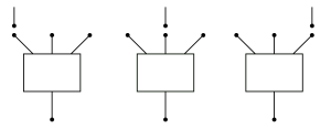
So we need to make sure we look for all possible trees.  As we get to the higher $A – \infty$ maps the space of all possible trees gets complicated.

Secondly, we need to start keeping track of the length of interior edges.  Each parametrizes a flow line, so we need to know exactly how long the partial flow line is that we want to parametrize.  This hasn’t been a problem because up to now, every flow line we considered had at least one noncompact end, because one end was asymptotic to a critical point, so its length was infinite.

We can solve both these problems by realizing that we can form a moduli space of italics(metric trees), an approach originally due to Stasheff.  Luckily, if we are careful, the moduli space is just some affine space for some dimension .

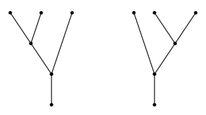
Embed the tree in the unit disk with the exterior vertices (the 1-valent vertices which map to critical points) cyclically ordered along the boundary.  Furthermore, assume that no vertex has valence 2, as this corresponds to a broken flow line, which we will consider separately later on.  The [exterior] edges will be those connected to the boundary and [interior] edges will be any other edge.  Assign a positive real number to each interior edge (the exterior edges are assumed to have length ).  Then the lengths of the interior edges, of which there can be at most , where is the number of exterior vertices, identify parametrize the moduli space and identify it with .  Call this space

For example, suppose , which is the relevant space for the .  The tree on the left corresponds to and the tree on the right corresponds to .

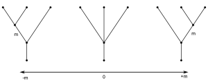
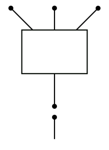
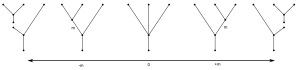
The space of metric trees is not compact but it can also be compactified, in the sense that as the length of the interior edge goes off to , the tree breaks into two metric trees.  For , this is just the union of a two 3-leaf Y trees.

For higher , it will break into two trees with and exterior vertices, respectively.  Again, we see the principle that a moduli space can be compactified using the product of lower-dimensional moduli spaces of the same type of object.

Choose four Morse functions such that their differences $f_i-f_j$ are collectively generic.  Let denote the moduli of metric trees with 4 exterior vertices parametrizing flow lines of the difference functions in the following way:  Each tree can be thought of as embedding in the unit disk and thus separates the disk into 4 regions.  Cyclically label each region with a function $f_i$.  Then an edge of a tree parametrizes a flow line of if it separates the regions labeled by and .  The trees can be oriented so  that every interior vertex has exactly one outgoing edge and exactly one exterior vertex has an incoming edge.  Assume that the oriented flows respect this orientation on edges.

The map is defined as follows.

In other words, count all rigid trees connecting to .

We’d now like to establish the relation

As with the , each term here describes one way a 1-dimensional tree could degenerate.  The first three correspond to an incoming flow line breaking:

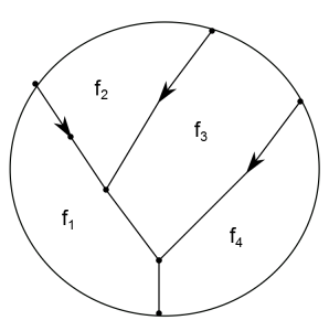
The last term corresponds to the outgoing flow line breaking:

And the terms involving correspond to an interior flow line breaking:

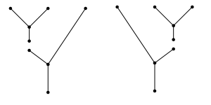
Again, the relation follows because each possible combination of broken trees can be glued to form the boundary of a 1-dimensional moduli space.  Moreover, each 1-dimensional tree must break/degenerate in one of the above ways.  Either an exterior edge breaks, which corresponds to the familiar compactification of Morse flow lines, or an interior breaks, which corresponds to the compactification of the moduli of metric trees.

Fukaya notes that this descends to Massey products on cohomology but I won’t go into that here.

The higher maps arise in the same way.  The map is defined by counting rigid trees with incoming and 1 outgoing edge.  The relation follows from the fact that each 1-dimensional tree breaks into two rigid trees.